| ID |
Date |
Author |
Subject |
|
13
|
Fri Aug 7 10:57:10 2020 |
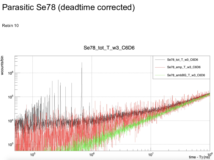
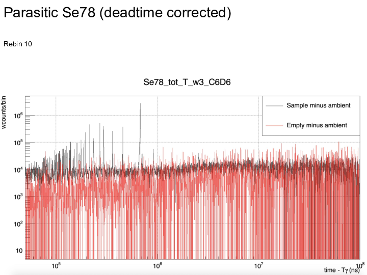
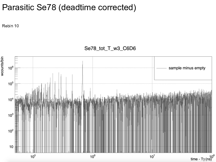
Ruchi | Monday meeting slides: 03 Aug |
|
| Attachment 1: 2020_08_03.pdf
|

|
|
6
|
Mon Jul 27 17:40:41 2020 |
Nikolay Sosnin | Meeting Slides (Calibrations + WFs) |
|
| Attachment 1: Broadening_Round1.pptx
|
| Attachment 2: Weighting_Gold.pptx
|
|
3
|
Fri Nov 3 15:06:51 2017 |
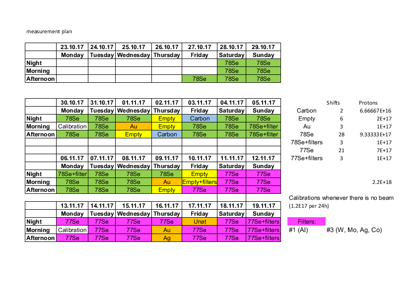
Claudia | Measurement Schedule updated |
|
| Attachment 1: measurementplan_new.pdf
|
|
|
5
|
Fri Jul 3 14:01:38 2020 |
Claudia | Link to Ruchi's list of runs + description |
https://docs.google.com/spreadsheets/d/1W1T2rC10UtOtrAaT8-ZAKFvX70v2PwDk_4-goYL-brI/edit?usp=sharing |
|
30
|
Thu Jun 29 09:21:13 2023 |
Annie | Info on Samples |
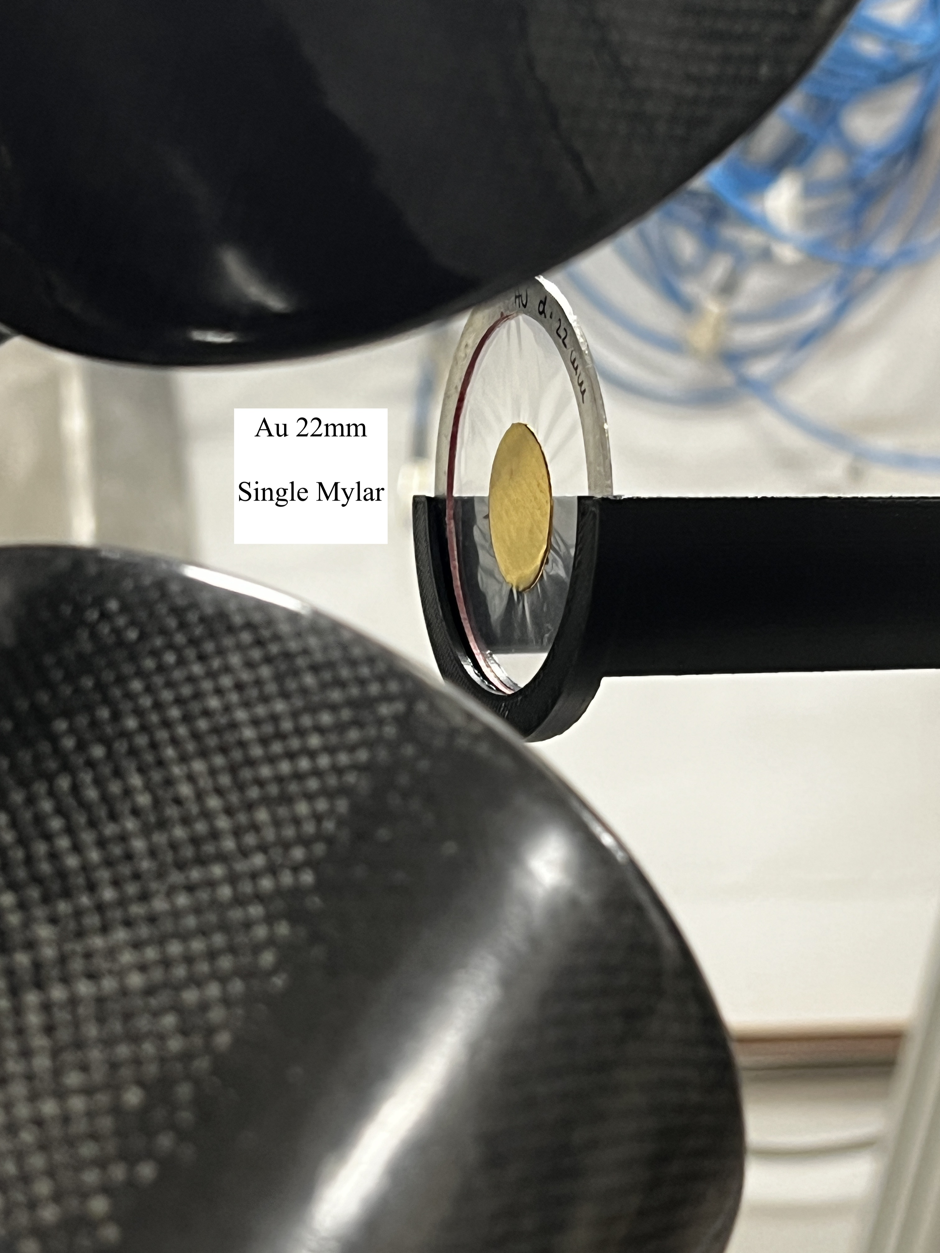
Both Au samples (20mm and 22mm) are single mylar.
Both Si30 (22mm) and natSi (20mm) are double mylar.
Empty is single mylar ONLY
Dummy is double mylar + glue |
| Attachment 1: IMG_2242.JPG
|

|
| Attachment 2: IMG_2248.JPG
|

|
| Attachment 3: IMG_2247.JPG
|
|
| Attachment 4: IMG_2246.JPG
|

|
|
66
|
Fri Jun 7 15:58:24 2024 |
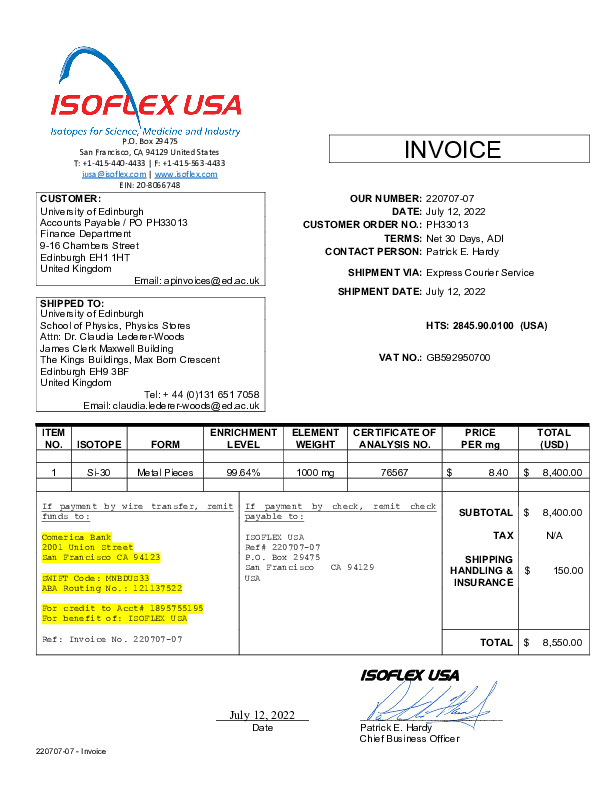
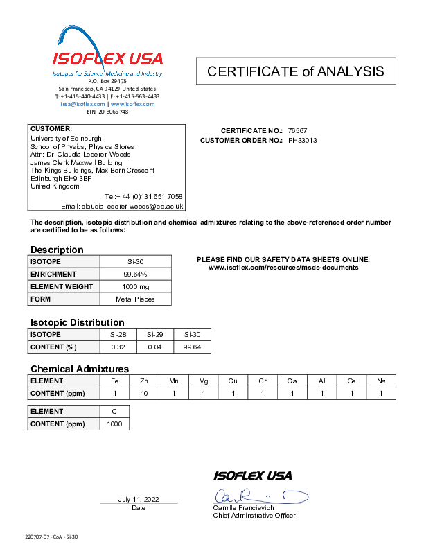
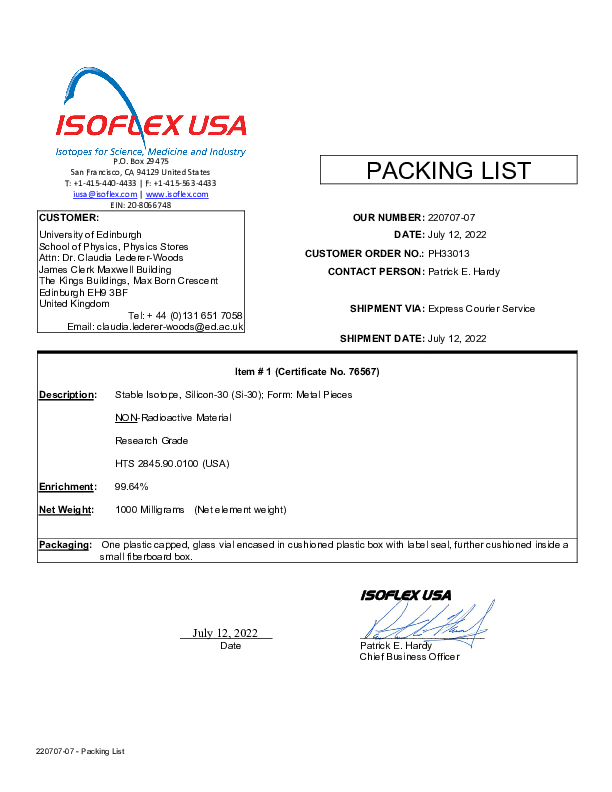
CLW | ISOFLEX Certificates for enriched Si samples |
Isoflex certificates for enriched silicon samples |
| Attachment 1: Si30_isoflex.pdf
|
|
| Attachment 2: 231226-01_-_Shipping_Documents(1).pdf
|
-0.png)
-1.png)
-2.png)
-3.png)
-4.png)
-5.png)
|
|
29
|
Thu Jun 22 10:37:39 2023 |
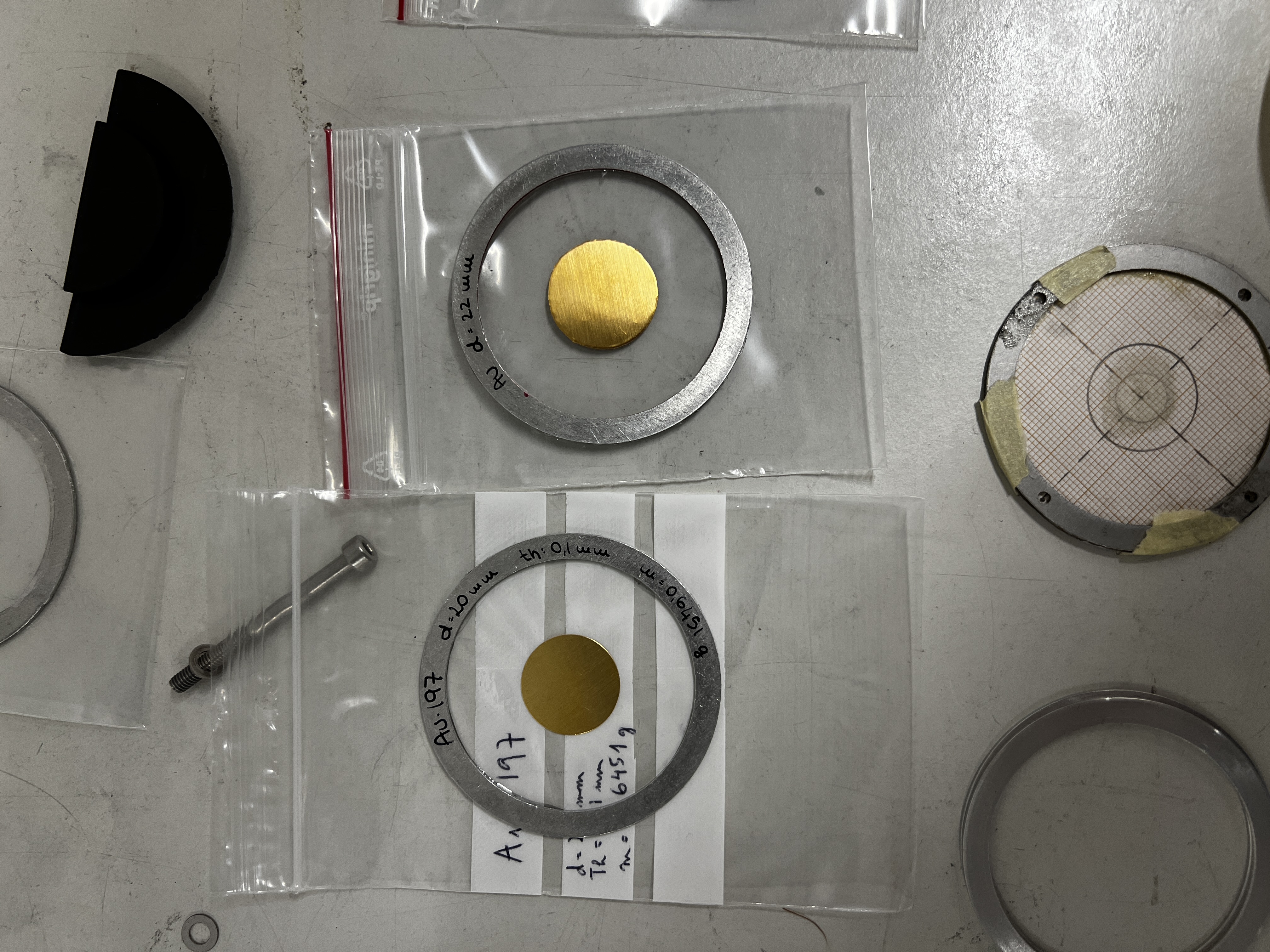
Annie | Gold 22mm Sample Images |
New 22mm sample compared to old 20mm sample used at the beginning of the campaign + picture of dummy target in the setup. |
| Attachment 1: IMG_2187.JPG
|

|
| Attachment 2: IMG_2186.JPG
|
|
| Attachment 3: IMG_2185.JPG
|

|
|
64
|
Thu Apr 4 09:50:36 2024 |
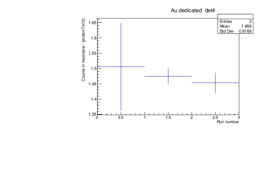
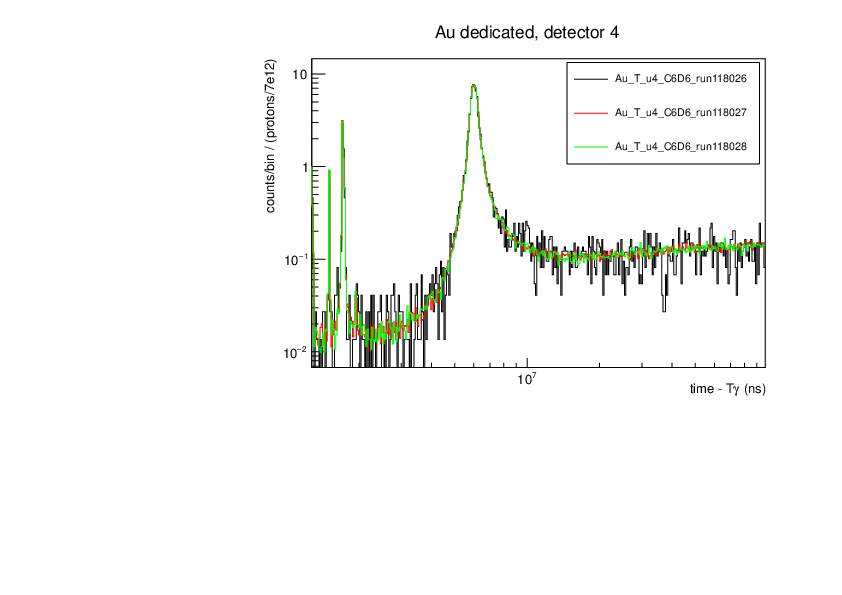
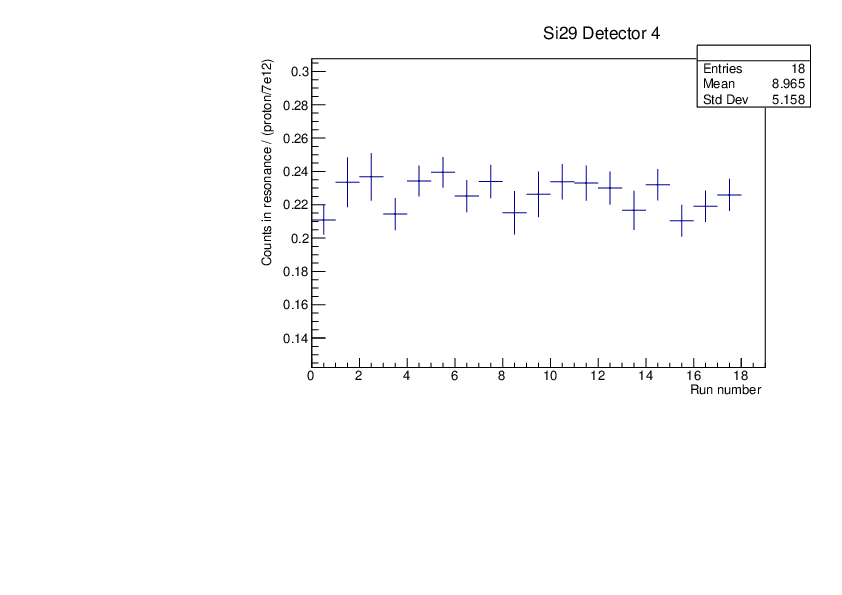
CLW | First Si analysis 2024 run |
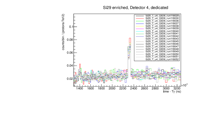
Au and Si29 runs normalised by proton number show consistency (dedicated pulses, example detector 4). Plots for tof spectra zooming on one resonance and histogram of counts in this resonance divided by protons with statistical errors.
Plots were produced with the macros attached. |
| Attachment 1: au_counts.pdf
|
|
| Attachment 2: au.pdf
|
|
| Attachment 3: si29_counts.pdf
|
|
| Attachment 4: si29.pdf
|
|
| Attachment 5: consistency.C
|
#include "TCanvas.h"
#include "TBrowser.h"
#include "TH2F.h"
#include "TH1F.h"
#include "TGraph.h"
#include "TGraphErrors.h"
#include "TMath.h"
#include <fstream>
#include "TFrame.h"
#include "TSystem.h"
#include "TLegend.h"
#include "TLegendEntry.h"
#include "TFile.h"
#include "TROOT.h"
#include "TStyle.h"
#include "TBox.h"
#include "TRandom.h"
#include "TObject.h"
#include "TObjString.h"
#include <iostream>
#include <cstdio>
#include <string>
#include <sstream>
#include "TLine.h"
#include "TTree.h"
#include "TBrowser.h"
#include "TF1.h"
#include <TStyle.h>
#include <THStack.h>
#include <TPad.h>
#include "TRandom.h"


void plot(){
    // replace this with name of your singles file
    TFile *f=new TFile("Single_Si29_ded.root","read");
    TString histo, norm, protons;

    ///file with a list of the histogram names for one detector
    // format Zn_T_u3_C6D6_runxxxxxx Zn_A_u3_SILI_runxxxxxx Zn_h_info_C6D6_runxxxxxx
    ifstream inni("Si29_C6D64_HistList.dat");
    TCanvas *c=new TCanvas();

    /// replace this with the tof around a resonance, i.e. binlow is the start of the resonance, binhigh is the end of the resonance
    // you can choose any resonance, best is a large one which is usally at big tof values
    /// this will be different for Au and for Zn.

float binlow=2250000;
float binhigh=2400000;

    TLegend *legend = new TLegend(0.65, 0.38, 0.89, 0.89);
    legend->SetBorderSize(1);
    legend->SetFillColor(0);
    legend->SetTextSize(0.03);
    int count2=0;
    int count_protons=0;


    //// replace this with the number of lines in your file "list"
int lines=59;

            float value[lines];
            float value2[lines];
            float valuesili[lines];
            float valuepkup[lines];
    float staterror[lines];
    while(1){

        inni>>histo>>norm>>protons;
        if ( ! inni ) break;


        char *s;
        if(count2==0) s="hist";
        if(count2>0)s="hist same";
        count2++;
        cout<<histo<<" "<<norm<<endl;


        TH1F *h=(TH1F*)f->Get(histo);
        //TH1F *hnorm=(TH1F*)f->Get(norm);
        TH1F *hpro=(TH1F*)f->Get(protons);


        int bin1=h->FindBin(binlow); //Ge70Bins
        int bin2=h->FindBin(binhigh);

        // this gives the total number of count in the resonance

        int counter2=h->Integral(bin1,bin2);


    value[count2-1]=float(counter2)/hpro->GetBinContent(4)*7E12;
        staterror[count2-1]=sqrt(float(counter2))/hpro->GetBinContent(4)*7E12;
             value2[count2-1]=float(counter2);
             valuesili[count2-1]=float(hpro->GetBinContent(4)/hpro->GetBinContent(8));
            valuepkup[count2-1]=float(hpro->GetBinContent(4)/hpro->GetBinContent(7));

        h->Scale(1/hpro->GetBinContent(4)*7E12);
        h->Rebin(50);
        h->SetLineColor(count2);
        h->DrawCopy(s);
        legend->AddEntry(h,histo, "l");
    }
    float sum=0;
    float weight=0;
     float weightsum=0;
    for(int i=0;i<count2;i++){

        weight=value2[i]/(value[i]*value[i]);

       sum=sum+value[i]*weight;


        weightsum=weightsum+weight;

        cout<<value[i]<<" "<<weight<<" "<<i<<endl;
    }


cout<< sum/weightsum <<endl;

    float deviation=0;
double stddev=0;

    for(int i=0;i<count2;i++){
        deviation=(sum/weightsum-value[i])/sum*weightsum*100;

stddev=(sum/weightsum-value[i])*(sum/weightsum-value[i])+stddev;

        cout<<" "<<deviation<<" % "<<sqrt(value2[i])/value2[i]*100<<" % counting "<<deviation/(sqrt(value2[i])/value2[i]*100)<< "   "<<i<<endl;
    }
    deviation=sqrt(1/count2*deviation);
    cout<<count2<<" "<<sum/count2<<endl;

double stddev2=sqrt(1/(float(count2-1))*stddev);

//STOP PROTON SCALING

cout<<"std dev is "<<stddev2/(sum/weightsum)*100<<" %"<<endl;
    legend->Draw();
cout<<"                                "<<endl;
    for(int i=0;i<count2;i++){

        cout<<" "<<valuesili[i]<<"  Prot/SILI    "<<valuepkup[i]<<"  Prot/PKUP   "<<valuesili[i]/valuepkup[i]<<" SILI/PKUP"<<endl;
    }


TH1F *hprosi=new TH1F("","",50,0,50);
TH1F *hprook=new TH1F("","",50,0,50);
TH1F *hsipk=new TH1F("","",50,0,50);
    TH1F *hcounts=new TH1F("","",50,0,50);

for(int i=0;i<count2;i++){
hprosi->SetBinContent(i+1,valuesili[i]);
hprook->SetBinContent(i+1,valuepkup[i]);
hsipk->SetBinContent(i+1,valuesili[i]/valuepkup[i]);
    hcounts->SetBinContent(i+1,value[i]);
    hcounts->SetBinError(i+1,staterror[i]);
    }

TCanvas *c3=new TCanvas;
c3->Divide(2,2);
c3->cd(1);
hprosi->Draw();
c3->cd(2);
hprook->Draw();
c3->cd(3);
hsipk->Draw();
    c3->cd(4);
    hcounts->Draw();


    TCanvas *c5=new TCanvas;
    hcounts->Draw();
}


void plotau(){
    // replace this with name of your singles file
    TFile *f=new TFile("Single_Au_ded.root","read");
    TString histo, norm, protons;

    ///file with a list of the histogram names for one detector
    // format Zn_T_u3_C6D6_runxxxxxx Zn_A_u3_SILI_runxxxxxx Zn_h_info_C6D6_runxxxxxx
    ifstream inni("Au_C6D64_HistList.dat");
    TCanvas *c=new TCanvas();

    /// replace this with the tof around a resonance, i.e. binlow is the start of the resonance, binhigh is the end of the resonance
    // you can choose any resonance, best is a large one which is usally at big tof values
    /// this will be different for Au and for Zn.

float binlow=12000000;
float binhigh=14000000;

    TLegend *legend = new TLegend(0.65, 0.38, 0.89, 0.89);
    legend->SetBorderSize(1);
    legend->SetFillColor(0);
    legend->SetTextSize(0.03);
    int count2=0;
    int count_protons=0;


    //// replace this with the number of lines in your file "list"
int lines=59;

            float value[lines];
            float value2[lines];
            float valuesili[lines];
            float valuepkup[lines];
    float staterror[lines];
    while(1){

        inni>>histo>>norm>>protons;
        if ( ! inni ) break;


        char *s;
        if(count2==0) s="hist";
        if(count2>0)s="hist same";
        count2++;
        cout<<histo<<" "<<norm<<endl;


        TH1F *h=(TH1F*)f->Get(histo);
        //TH1F *hnorm=(TH1F*)f->Get(norm);
        TH1F *hpro=(TH1F*)f->Get(protons);


        int bin1=h->FindBin(binlow); //Ge70Bins
        int bin2=h->FindBin(binhigh);

        // this gives the total number of count in the resonance

        int counter2=h->Integral(bin1,bin2);


    value[count2-1]=float(counter2)/hpro->GetBinContent(4)*7E12;
        staterror[count2-1]=sqrt(float(counter2))/hpro->GetBinContent(4)*7E12;
             value2[count2-1]=float(counter2);
             valuesili[count2-1]=float(hpro->GetBinContent(4)/hpro->GetBinContent(8));
            valuepkup[count2-1]=float(hpro->GetBinContent(4)/hpro->GetBinContent(7));

        h->Scale(1/hpro->GetBinContent(4)*7E12);
        h->Rebin(50);
        h->SetLineColor(count2);
        h->DrawCopy(s);
        legend->AddEntry(h,histo, "l");
    }
    float sum=0;
    float weight=0;
     float weightsum=0;
    for(int i=0;i<count2;i++){

        weight=value2[i]/(value[i]*value[i]);

       sum=sum+value[i]*weight;


        weightsum=weightsum+weight;

        cout<<value[i]<<" "<<weight<<" "<<i<<endl;
    }


cout<< sum/weightsum <<endl;

    float deviation=0;
double stddev=0;

    for(int i=0;i<count2;i++){
        deviation=(sum/weightsum-value[i])/sum*weightsum*100;

stddev=(sum/weightsum-value[i])*(sum/weightsum-value[i])+stddev;

        cout<<" "<<deviation<<" % "<<sqrt(value2[i])/value2[i]*100<<" % counting "<<deviation/(sqrt(value2[i])/value2[i]*100)<< "   "<<i<<endl;
    }
    deviation=sqrt(1/count2*deviation);
    cout<<count2<<" "<<sum/count2<<endl;

double stddev2=sqrt(1/(float(count2-1))*stddev);

//STOP PROTON SCALING

cout<<"std dev is "<<stddev2/(sum/weightsum)*100<<" %"<<endl;
    legend->Draw();
cout<<"                                "<<endl;
    for(int i=0;i<count2;i++){
... 36 more lines ...
|
| Attachment 6: List_Formatter.cpp
|
// g++ -Wall -O3 -g List_Formatter.cpp -o List_Formatter && ./List_Formatter

#include <iostream>
#include <fstream>
#include <sstream>
#include <string>
#include <vector>

using namespace std;

int main(){

	string sample_name = "Au"; //A prefix for the TTOFSort output file histogram names, e.g. Zn1 is the first block of zinc runs

    int runlist[]={118026, 118027, 118028, -1};

	for(int detn = 1; detn <= 4; detn++){ //Loop over 4 C6D6 detectors

		string outname = sample_name; //Create output file name in the format Sample_C6D6#_HistList.dat
		outname += "_C6D6";
		stringstream formatter;
		formatter << detn;
		outname += formatter.str(); //This string stream now contains detector name integer converted to string
		outname += "_HistList.dat";

		ofstream ofile;
		ofile.open(outname.c_str());
		if(!ofile.is_open()){cout << "ERROR: Cannot open output file " << outname << endl; return 0;}

		for(int run_index = 0; run_index < (int)(sizeof(runlist) / sizeof(int)); run_index++){ //Loop over each of the runs

			if(runlist[run_index] != -1){

				stringstream run_str;
				run_str << runlist[run_index]; //Save run number as string

				string histname1 = sample_name;
				histname1 += "_T_u";
				histname1 += formatter.str();
				histname1 += "_C6D6_run";
				histname1 += run_str.str();

				string histname2 = sample_name;
				histname2 += "_A_u";
				histname2 += formatter.str();
				histname2 += "_SILI_run";
				histname2 += run_str.str();

				string histname3 = sample_name;
				histname3 += "_h_info_C6D6_run";
				histname3 += run_str.str();

				run_str.str(""); //Clear the stringstream

				ofile << histname1 << " " << histname2 << " " << histname3 << endl;
			}
		}

		formatter.str(""); //Clear the stringstream

		ofile.close();
	}

	return 0;
}
|
|
26
|
Fri Jul 29 17:21:47 2022 |
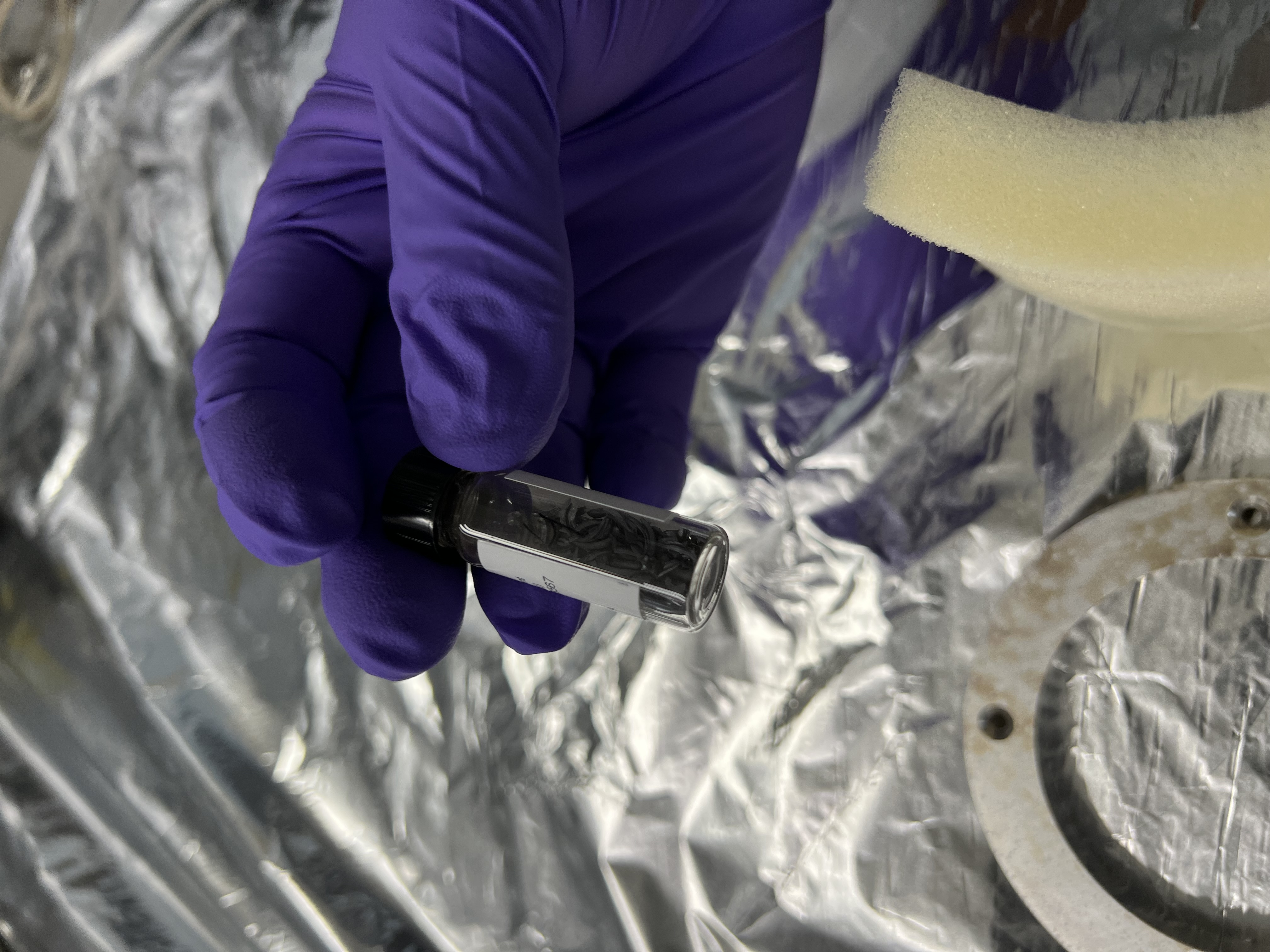
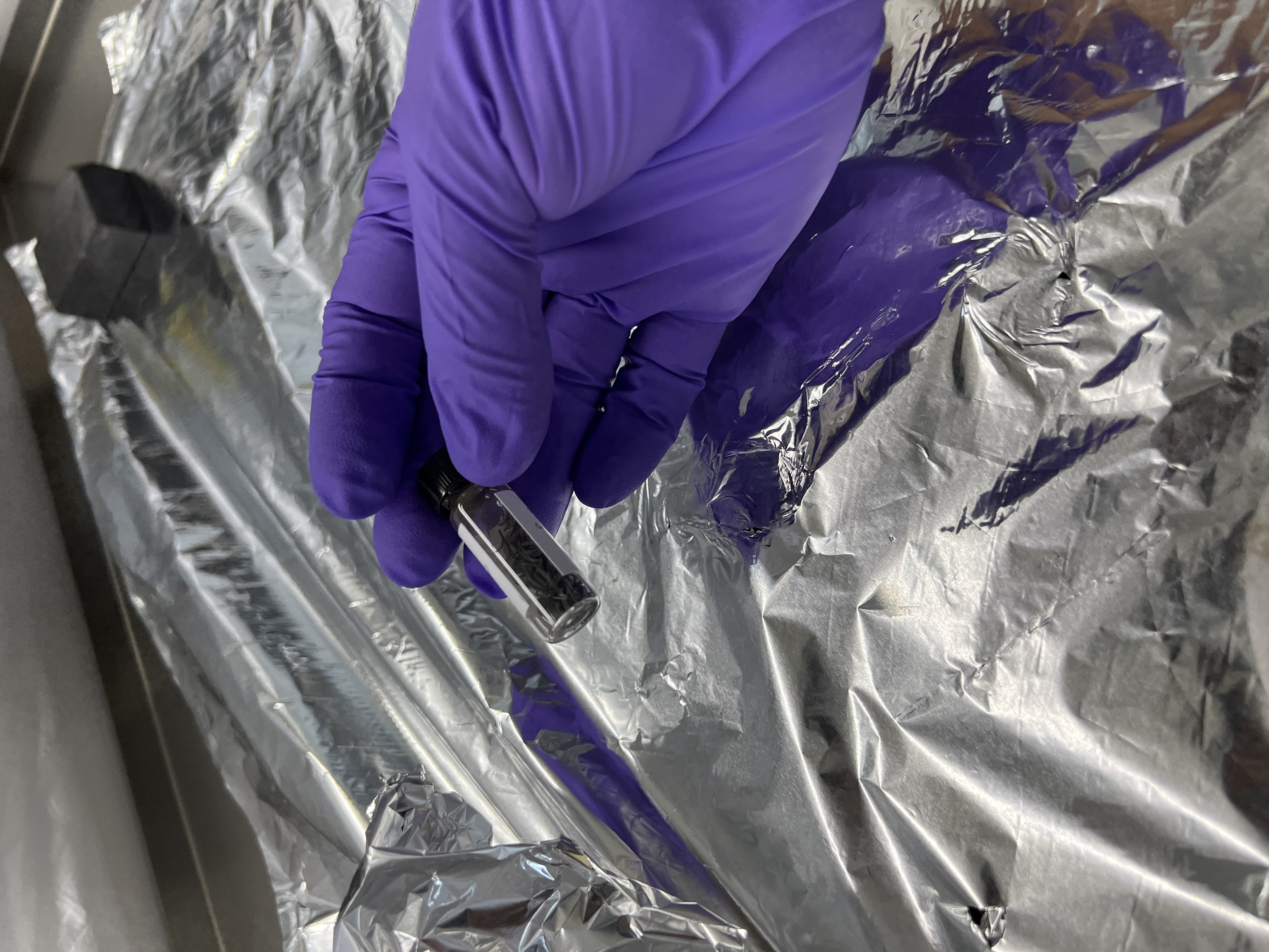
Ragan | Enriched Si-30 |
Attached are the pictures of enriched Si-30 metal pieces. |
| Attachment 1: IMG_2692.jpg
|
|
| Attachment 2: IMG_2693.jpg
|
|
|
41
|
Fri Jul 28 12:19:10 2023 |
Michael Donnachie | EAR2 consistency checks, PKUP BCT SILI and normalised counts |
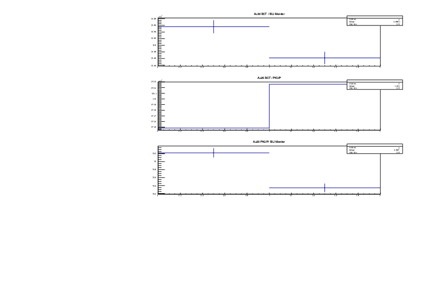
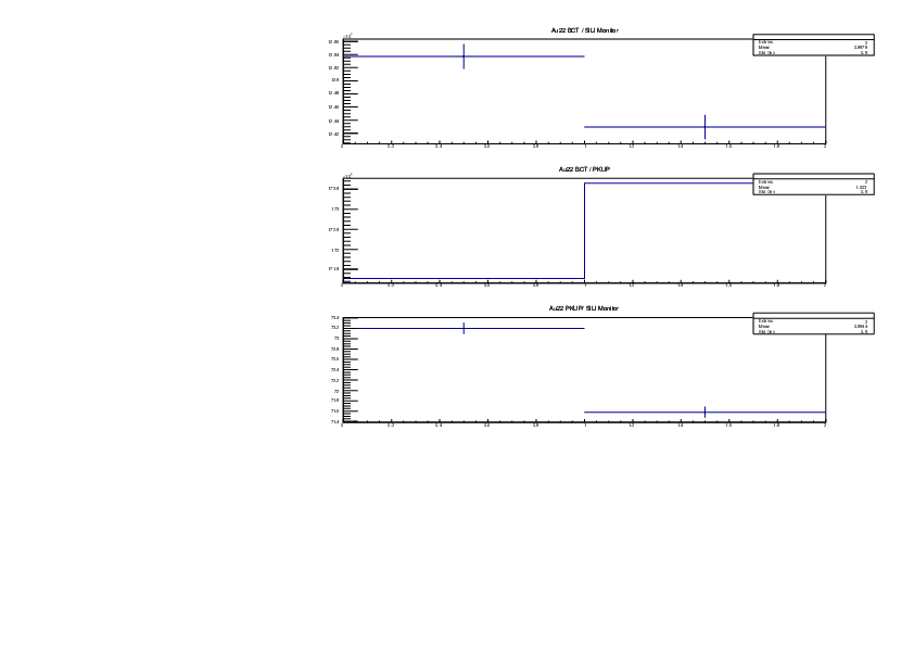
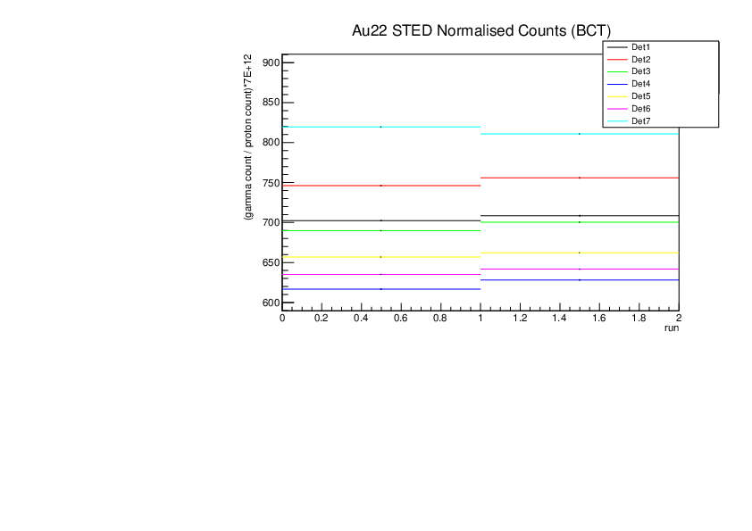
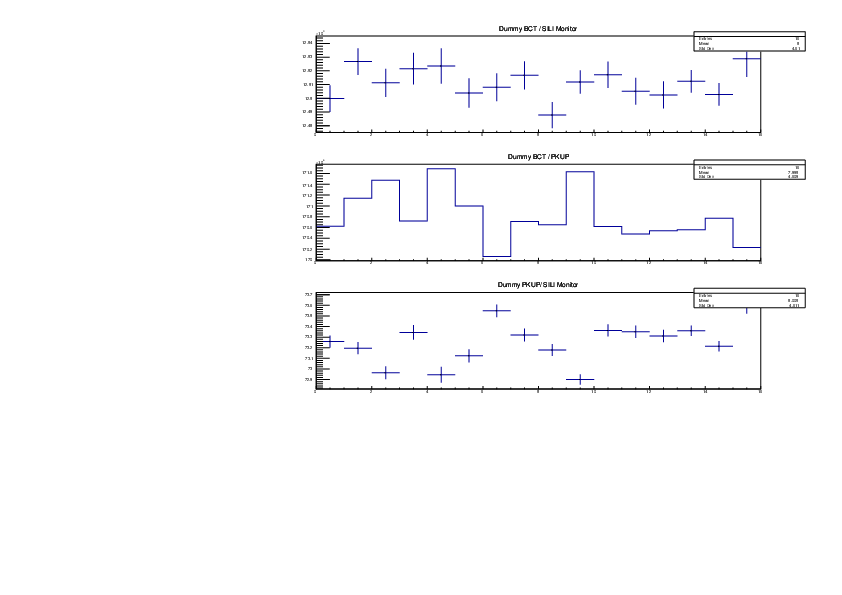
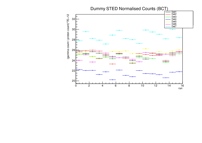
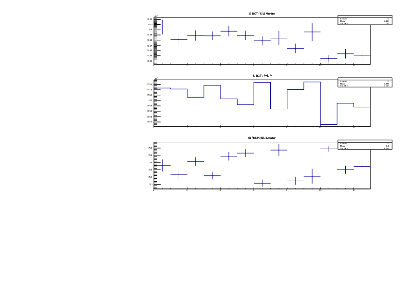
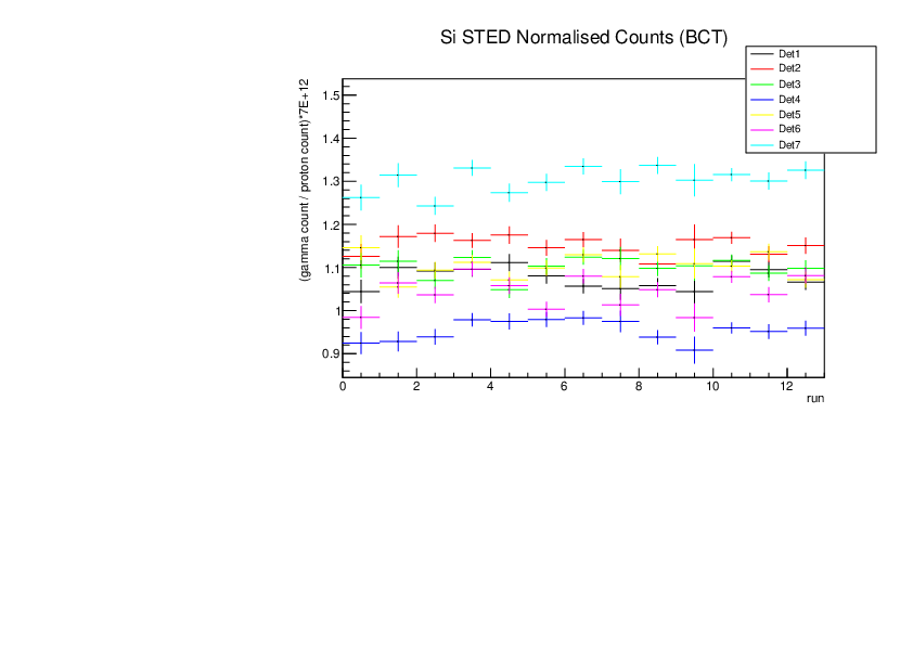
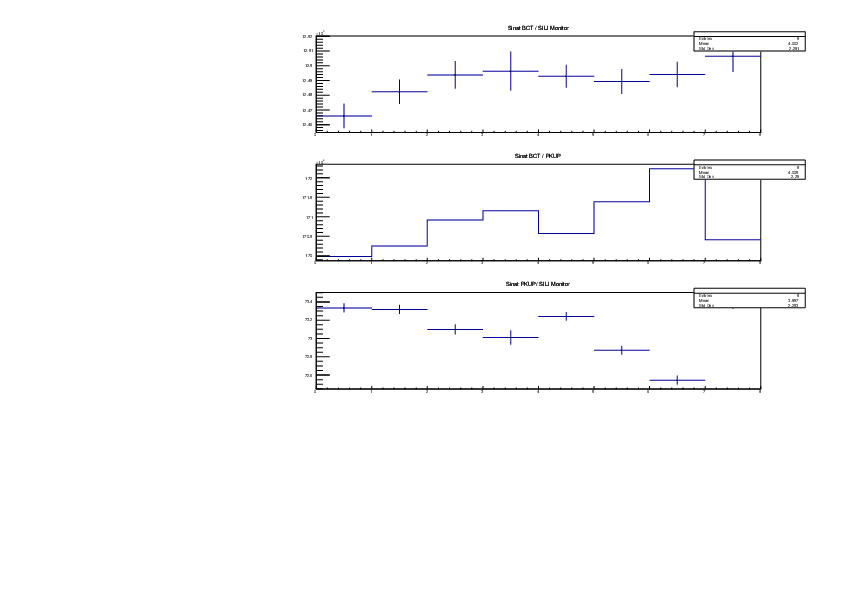
The EAR2 ratios of BCT/PKUP, BCT/SILI and PKUP/SILI plotted for each run for samples Si, Sinat, Au20, Au22 and Dummy.
Also included is the normalised counts (counts/BCT) with 7 detectors on one plot (STED8 was ommited). 'counts' for Si was integreated over the Si resonance, for Au it was integrated over the largest resonance. For Dummy and Sinat the counts were integrated over a large range of 1e+4 to 1e+6ns. The Sinat resonance was too small for adequate statistics to only integrate over the resonance hence why a large range was used. The C6D6 normalised counts were not plotted as there seems to be issues with this detector in EAR2.
|
| Attachment 1: Au20_Ratios.pdf
|
|
| Attachment 2: Au20_STED_normalised_counts.pdf
|

|
| Attachment 3: Au22_Ratios.pdf
|
|
| Attachment 4: Au22_STED_normalised_counts.pdf
|
|
| Attachment 5: Dummy_Ratios.pdf
|
|
| Attachment 6: Dummy_STED_normalised_counts.pdf
|
|
| Attachment 7: Si_Ratios.pdf
|
|
| Attachment 8: Si_STED_normalised_counts.pdf
|
|
| Attachment 9: Sinat_Ratios.pdf
|
|
| Attachment 10: Sinat_STED_normalised_counts.pdf
|

|
|
42
|
Mon Jul 31 12:00:02 2023 |
Nikolay Sosnin | EAR2 Silicon Samples |
|
| Attachment 1: EAR2_30Si.JPG
|

|
| Attachment 2: EAR2_Sinat_Closeup.JPG
|

|
| Attachment 3: Goodfellow_Sinat_Sample.JPG
|

|
| Attachment 4: Laser_Alignment.JPG
|
|
|
44
|
Mon Aug 28 12:21:09 2023 |
Michael Donnachie | EAR2 STED Calibration Parameters |
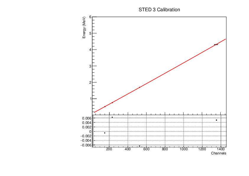
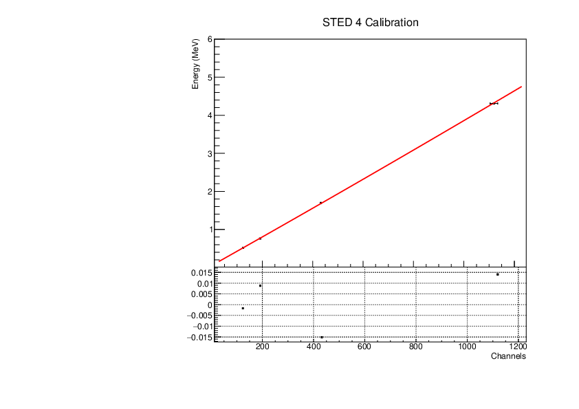
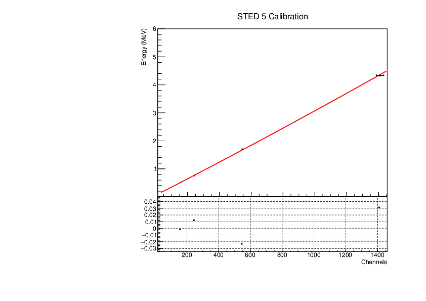
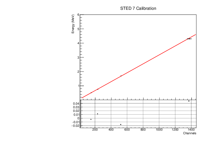
Calibration parameters for each STED detector: With function f=p0+p1*x+p2*x*x
|
Detector
|
p0 Value |
p0 Error |
p1 Value |
p1 Error |
p2 Value |
p2 Error |
|
STED 1
|
5.67257E-02 |
|
|
|
|
6.80573E-08 |
| STED 2 |
|
|
|
|
|
7.35018E-08 |
| STED 3 |
|
|
|
|
|
5.55624E-08 |
| STED 4 |
|
|
|
|
|
7.71976E-08 |
| STED 5 |
|
|
|
|
|
5.75051E-08 |
| STED 6 |
|
|
|
|
|
5.06241E-08 |
| STED 7 |
|
|
|
|
|
5.79147E-08 |
A quadratic function was fitted to the reference point channel (from experimental histogram) and reference point energy (from simulation histogram). The reference point 'r' was r=mean+(FWHM/2) for a gaussian fitted to each compton edge. A quadratic function was used as it fitted the higher energy AmBe reference point better than a linear function. This is highlighted by the comparisson of "STED 2 Calibration" and "STED 2 Example Linear Fit Calibration" plots below. The p0 error is quite large and p2 error very large (larger than the parameter value in STED1) - however the parameters are highly correlated which may have inflated the error.
CmC histograms were not used as the compton edge could not be located.
For reference the STED 1 correlation matrix:
| |
p0 |
p1 |
p2 |
| p0 |
1 |
-0.92473 |
0.78779 |
| p1 |
-0.92473 |
1 |
-0.91714 |
| p2 |
0.78779 |
-0.91714 |
1 |
|
| Attachment 1: Example_STED2_calibration.pdf
|

|
| Attachment 2: STED1_calibration.pdf
|

|
| Attachment 3: STED2_calibration.pdf
|

|
| Attachment 4: STED3_calibration.pdf
|
|
| Attachment 5: STED4_calibration.pdf
|
|
| Attachment 6: STED5_calibration.pdf
|
|
| Attachment 7: STED6_calibration.pdf
|

|
| Attachment 8: STED7_calibration.pdf
|
|
|
45
|
Mon Aug 28 14:07:23 2023 |
Michael Donnachie | EAR2 Experiment vs Simulated Amplitude Spectrums |
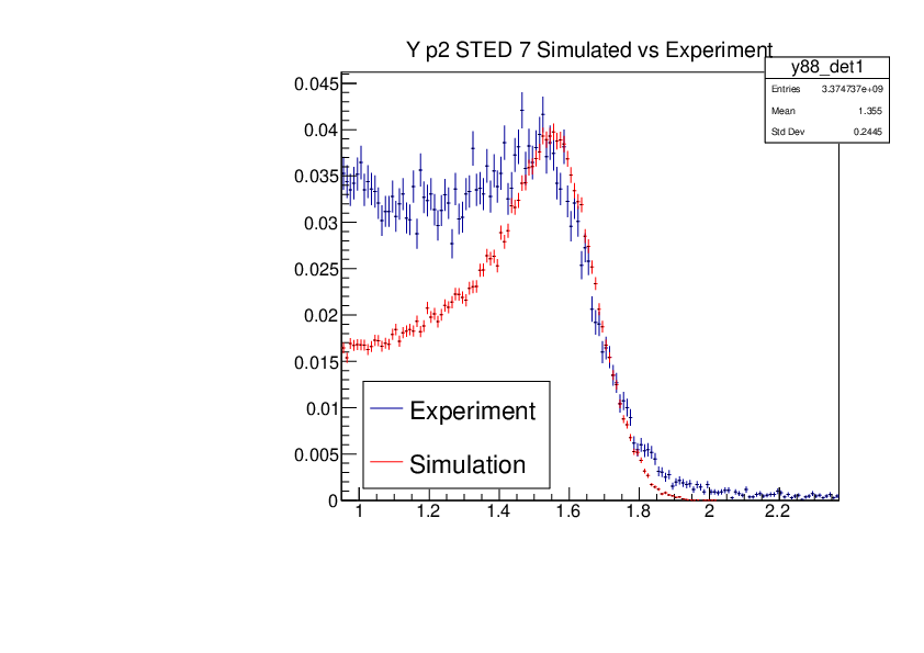
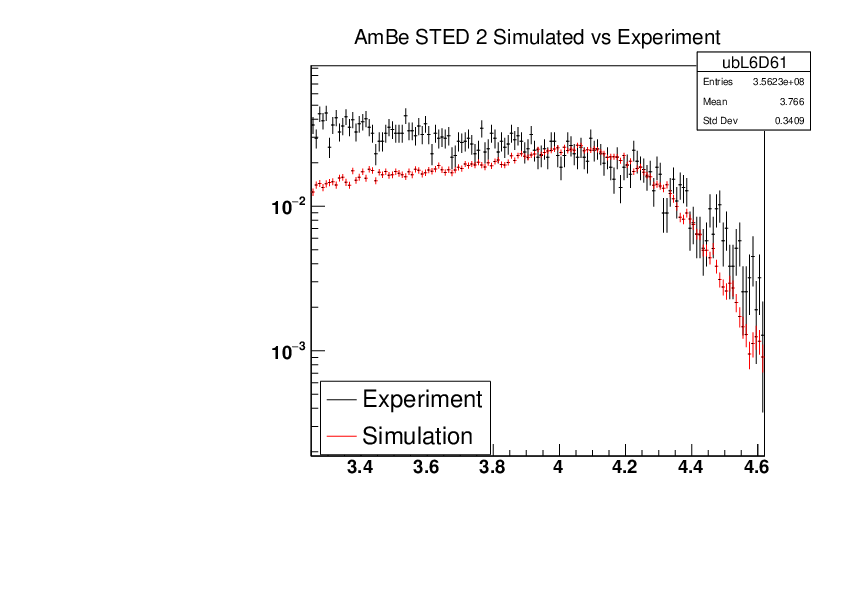
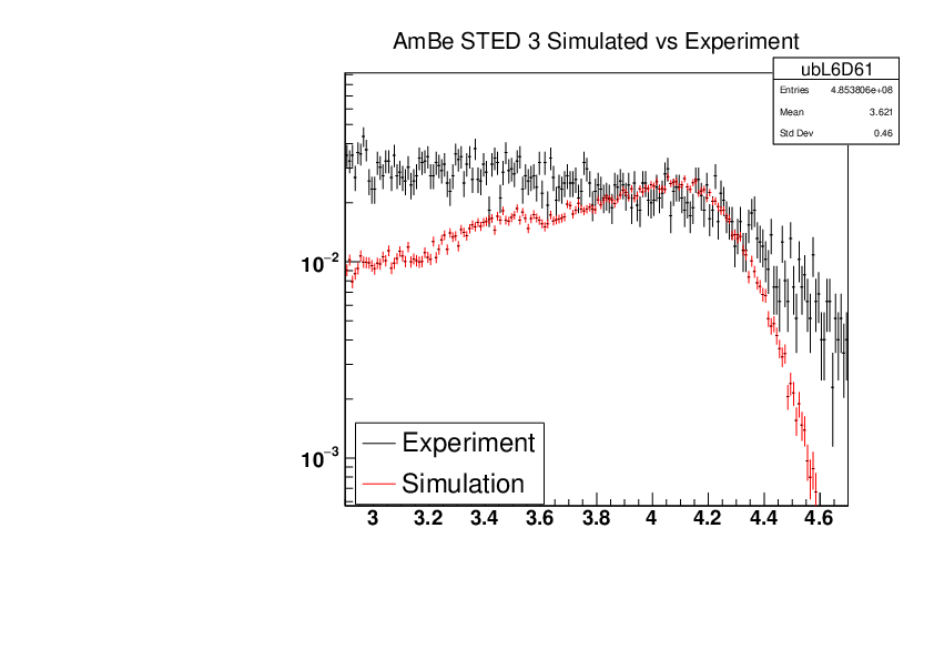
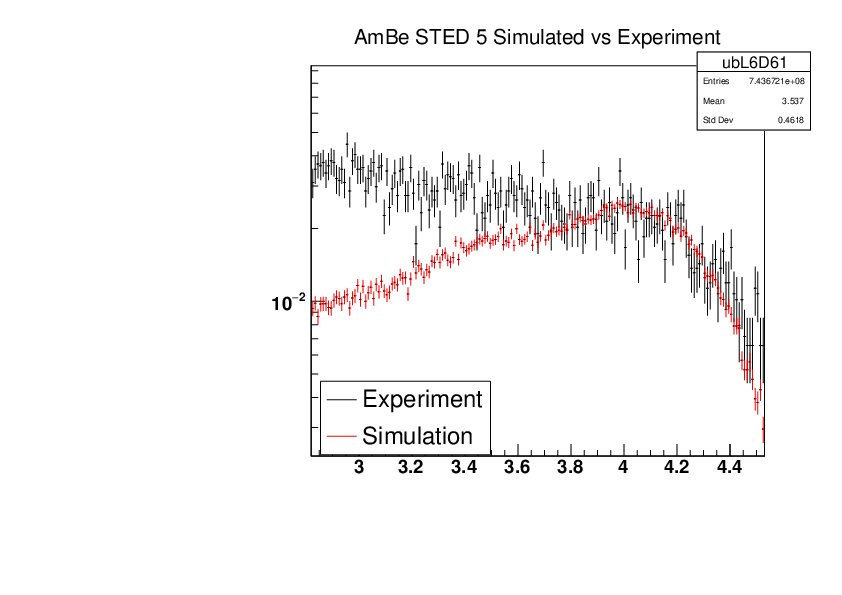
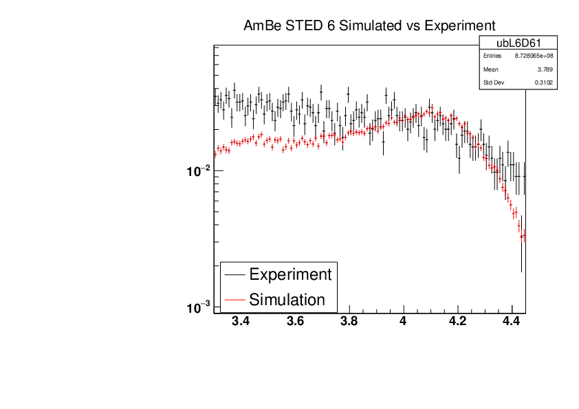
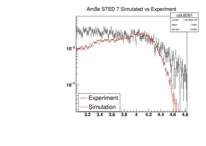
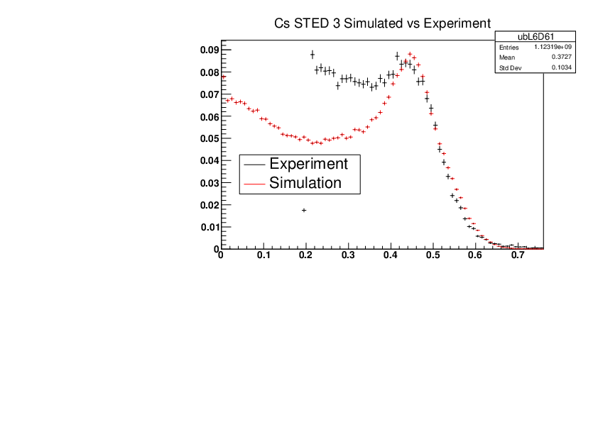
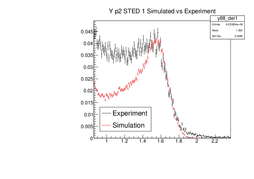
Attatched are the overlayed compton edges for the calibrated experimental and the GEANT4 simulations. Note p1 and p2 denotes the lower and higher energy compton edges for Yttrium.
The experimental and simulated histograms are shifted in quite a few of these plots suggesting the calibration was not fully successful. The compton edge for AmBe was difficult to locate and may have contributed to the poor calibration. |
| Attachment 1: YP2_STED5_Experiment_vs_Simulated.pdf
|

|
| Attachment 2: YP2_STED6_Experiment_vs_Simulated.pdf
|

|
| Attachment 3: YP2_STED7_Experiment_vs_Simulated.pdf
|
|
| Attachment 4: AmBe_STED1_Experiment_vs_Simulated.pdf
|

|
| Attachment 5: AmBe_STED2_Experiment_vs_Simulated.pdf
|
|
| Attachment 6: AmBe_STED3_Experiment_vs_Simulated.pdf
|
|
| Attachment 7: AmBe_STED4_Experiment_vs_Simulated.pdf
|

|
| Attachment 8: AmBe_STED5_Experiment_vs_Simulated.pdf
|
|
| Attachment 9: AmBe_STED6_Experiment_vs_Simulated.pdf
|
|
| Attachment 10: AmBe_STED7_Experiment_vs_Simulated.pdf
|
|
| Attachment 11: Cs_STED1_Experiment_vs_Simulated.pdf
|

|
| Attachment 12: Cs_STED2_Experiment_vs_Simulated.pdf
|

|
| Attachment 13: Cs_STED3_Experiment_vs_Simulated.pdf
|
|
| Attachment 14: Cs_STED4_Experiment_vs_Simulated.pdf
|

|
| Attachment 15: Cs_STED5_Experiment_vs_Simulated.pdf
|

|
| Attachment 16: Cs_STED6_Experiment_vs_Simulated.pdf
|

|
| Attachment 17: Cs_STED7_Experiment_vs_Simulated.pdf
|

|
| Attachment 18: YP1_STED1_Experiment_vs_Simulated.pdf
|

|
| Attachment 19: YP1_STED2_Experiment_vs_Simulated.pdf
|

|
| Attachment 20: YP1_STED3_Experiment_vs_Simulated.pdf
|

|
| Attachment 21: YP1_STED4_Experiment_vs_Simulated.pdf
|

|
| Attachment 22: YP1_STED5_Experiment_vs_Simulated.pdf
|

|
| Attachment 23: YP1_STED6_Experiment_vs_Simulated.pdf
|

|
| Attachment 24: YP1_STED7_Experiment_vs_Simulated.pdf
|

|
| Attachment 25: YP2_STED1_Experiment_vs_Simulated.pdf
|
|
| Attachment 26: YP2_STED2_Experiment_vs_Simulated.pdf
|

|
| Attachment 27: YP2_STED3_Experiment_vs_Simulated.pdf
|

|
| Attachment 28: YP2_STED4_Experiment_vs_Simulated.pdf
|

|
|
40
|
Fri Jul 28 12:07:33 2023 |
Michael Donnachie | EAR2 C6D6 timeshift issues |
There seems to be issues with the EAR2 C6D6 T histograms. For Au the earlier run seems to be shifted for detector 2 compared to the rest.
For Si plotted is 3 different runs 216123, 216128 and 216135 for both detectors. The histogram is messy but highlights that there is a problem. The single Si resonace should be around 20 000ns and this is only the case for run216128.
Apologies for no legend on plots.
Au22
det1 run216158 black
det1 run216109 red
det2 run216158 green
det2 run216109 blue
Au22
det1 run216157 black
det1 run216108 red
det2 run216157 green
det2 run216108 blue
|
| Attachment 1: Au20_C6D6_both_det_timeshift.pdf
|

|
| Attachment 2: Au22_C6D6_both_det_timeshift.pdf
|

|
| Attachment 3: Si30_C6D6_bothdet_3runs.pdf
|

|
|
46
|
Tue Aug 29 10:32:35 2023 |
Michael Donnachie | EAR1 Parasitic vs Dedicated runs |
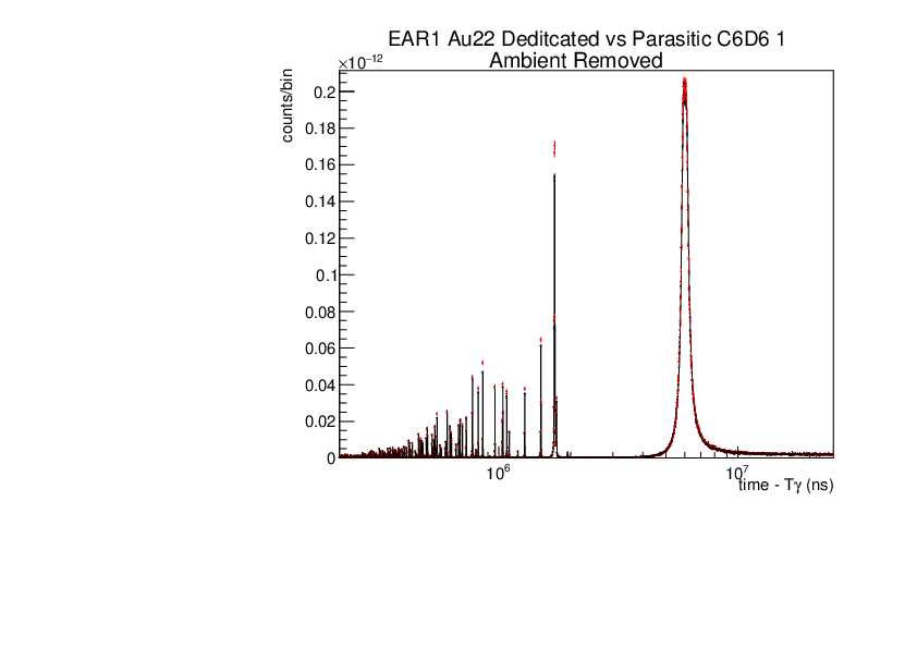
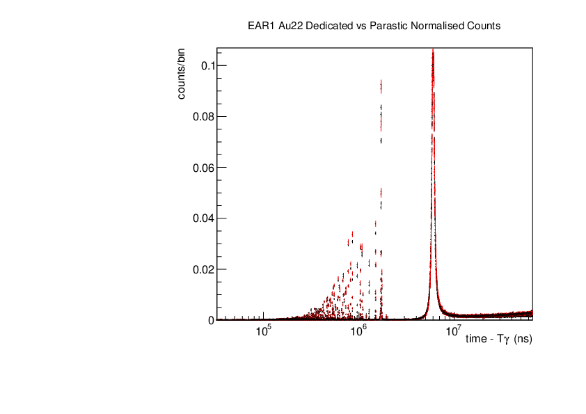
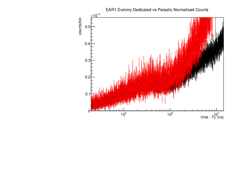
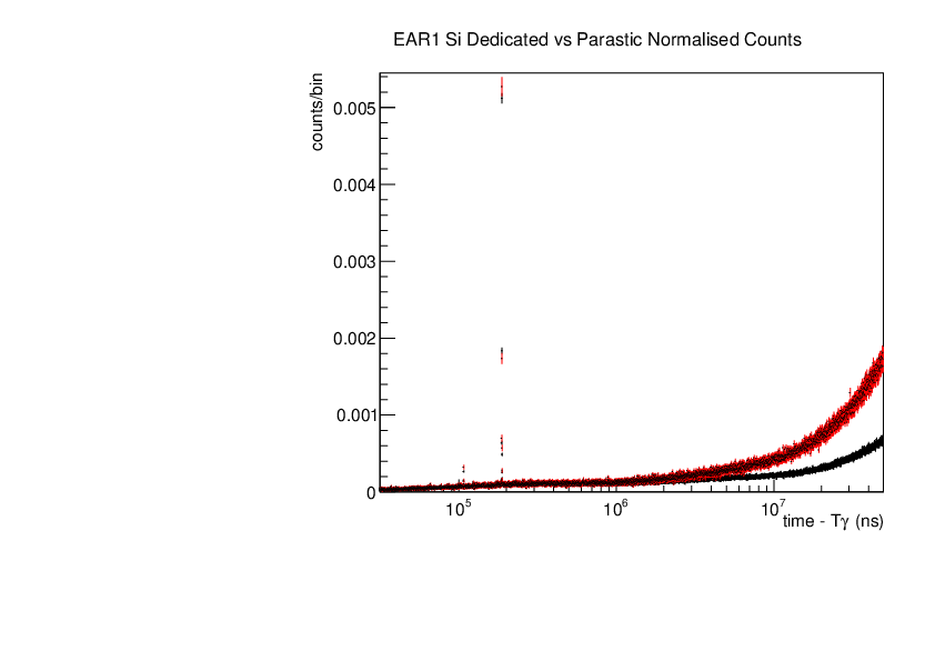
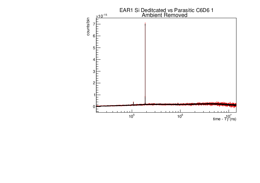
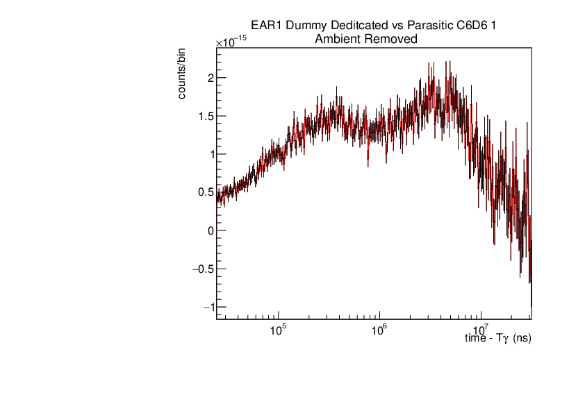
Below are the histograms of parasitic vs dedicated runs for EAR1. Also included are histograms with ambient background removed which closes the gap between parasitic and dedicated histograms. This was preformed by scaling the ambient by counts by a multiplication of (dedicated or parasitic) bunch number/ambient bunch number. There are no legends but the dedicated counts are in black and parasitic counts in red. Only included are C6D6 1 detectors but the other three detectors were equivelant.
|
| Attachment 1: Au22_large_range_ambrem_A.pdf
|
|
| Attachment 2: Au22_large_range.pdf
|
|
| Attachment 3: Dummy_large_range.pdf
|
|
| Attachment 4: Si_large_range.pdf
|
|
| Attachment 5: Si_Resonance_ambrem_B.pdf
|
|
| Attachment 6: Dummy_large_range_ambrem.pdf
|
|
|
56
|
Wed Nov 15 13:40:50 2023 |
Claudia | Determination of neutron capture yield and related corrections |
Here are all the files needed for calculation of the yield. There is some information that still needs to be added to the energyandyield.c file, for example the atomic mass of your target in amu, the neutron separation energy for the compound nucleus in MeV (this is needed due to using the Weighting technique). Also, you need to add some lines to read the tof histogram, which will then be converted in a neutron energy hisogram and then divided by the flux.
For the conversion to neutron energy we assume an approximate flight path for now. We will determine this more accurately once we have the yields and fit resonances. Emma will need to use a different flux than Annie, because we have a different spallation target. Emma's flux is preliminary, so we also should look at the SILI detectors at some point.
There are some more instances where names for rootfiles and ascii files need to be added. In the first instance, please try and add the missing information and try running the code. I haven't tested it so there may be still problem. To run it you will need to download the 3 rootfiles into the same folder (or move somewhere else and adjust the path name in the .c file.
PLEASE set variable THRESHSCALER to 1 for now. We dont know yet what it is :-) |
| Attachment 1: evalFlux_prelim.root
|
| Attachment 2: nTOF-Ph2_fluence_2009-2011_6Dec2011.root
|
| Attachment 3: BIF_2011_norm.root
|
| Attachment 4: energyandyield.c
|
#include "TCanvas.h"
#include "TBrowser.h"
#include "TH2F.h"
#include "TH1F.h"
#include "TGraph.h"
#include "TGraphErrors.h"
#include "TMath.h"
#include <fstream>
#include "TFrame.h"
#include "TSystem.h"
#include "TLegend.h"
#include "TLegendEntry.h"
#include "TFile.h"
#include "TROOT.h"
#include "TStyle.h"
#include "TBox.h"
#include "TRandom.h"
#include "TObject.h"
#include "TObjString.h"
#include <iostream>
#include <cstdio>
#include <string>
#include <sstream>
#include "TLine.h"
#include "TTree.h"
#include "TBrowser.h"
#include "TF1.h"
#include <TStyle.h>
#include <THStack.h>
#include <TPad.h>
#include "TRandom.h"


using namespace std;

TH1F *toftoene_fixedbin(TH1F *htof,Double_t L,Double_t offset,Int_t binoffset);
void WriteHistogramFile(TString filename,TH1F *h);

float Sn= 0  ; // neutron separation energy in MeV
float Amass= 0; // mass of your nucleus in atomic mass units

/// L flight path in cm, assumed
/// offset ... any offset in time of flight from daq (N/A here, hence 0)
/// binoffset this is just to exclude very low tof bins which are at too high energy to be of interest 10000 should be ok

void run(){

    /// LOAD TIME OF FLIGHT SPECTRUM

    TH1F *hene=toftoene_fixedbin(NAMEOFTOFSPECTRUM,18500,0,10000);


    hene->Draw();  /// draw tof histogram concerted to energy

    TH1F *h_me=(TH1F*)hene->Clone();

    //// NOW moving on to division by flux
     /// the neutron flux is given per bunch assuming a standard proton intensity of 7E12 protons / bunch. Hence the division is by no of protons and then multiplied by 7E12 to get to the number of standard bunches


   h_me->Scale(1/(h_mon->GetBinContent(4)/7E12));


    /// file that contains the neutron flux. We are looking at the flux in isolethargic units
    TFile *fflux = new TFile("nTOF-Ph2_fluence_2009-2011_6Dec2011.root", "read"); //for EMMA: evalFlux_prelim.root

    TH1F *sim = (TH1F*)fflux->Get("hNFluenceEVALUATED2011"); // FOR EMMA: hEval_Abs

    //Neutron flux that is independent of the binning of the histogram. The number of neutrons between E1 and E1 can be found by multiplying the value in the histogram by the logarithmic bin width, i.e. log(E2)-log(E1)

        TH1F *yield1 = (TH1F*)h_me->Clone();

        cout<<"DIVIDE BY FLUX"<<endl;
        for(Int_t i=1; i<=h_me->GetNbinsX(); i++)
        {

            float auxbin1 = sim->FindBin(h_me->GetBinCenter(i));  // find the bin in the flux histogram
            float scaler1 = TMath::Log(h_me->GetBinLowEdge(i+1)/h_me->GetBinLowEdge(i)); // determine the binwidth of count histogram

            yield1->SetBinContent(i,h_me->GetBinContent(i)/(sim->GetBinContent(auxbin1)*scaler1));
            // this is the division by the flux. The number of coutns gets divided by the number of neutrons in that particular bin

            if(sim->GetBinContent(auxbin1)<=0)yield1->SetBinContent(i,0); // this is in case the flux histgram has a content <=0, so we do not divide by a negative or 0

             if(sim->GetBinContent(auxbin1)>0){

            float binerr_rel=sqrt(pow(h_me->GetBinError(i)/h_me->GetBinContent(i),2) + pow(sim->GetBinError(auxbin1)/sim->GetBinContent(auxbin1),2));

                 // this calculates the relative uncertainty taking into consideration the sample uncertainties and the uncertaities in the flux histogram

            float binerr=binerr_rel*yield1->GetBinContent(i);
                  // calculation of absolute uncertainty

            if(h_me->GetBinContent(i)==0)binerr=h_me->GetBinError(i)/(sim->GetBinContent(auxbin1)*scaler1);
                 /// this is again to avoid divition by  0

            yield1->SetBinError(i,binerr);
            }


        }


        for(int g=1;g<=h_me->GetNbinsX();g++)
        {
    yield1->SetBinContent(g,yield1->GetBinContent(g)*threshscaler/(Sn+  Amass/(1.0086649+Amass)*yield1->GetBinCenter(g)/1e6));
    yield1->SetBinError(g,yield1->GetBinError(g)*threshscaler/(Sn+  Amass/(1.0086649+Amass)*yield1->GetBinCenter(g)/1e6));
    }


   // this is an additional correction since the neutron beam size varies slightly with neutrom energy. Emma, you can skip that for now as it will be different for you, and we dont have that information yet.

        cout << "BIF CORRECTION" <<endl;

        TFile *bif=new TFile("BIF_2011_norm.root","read");
        TH1F *hbif=(TH1F*)bif->Get("histo");


        for(int f=1;f<=yield1->GetNbinsX();f++){
            float center=yield1->GetBinCenter(f);
            int binni=hbif->FindBin(center);

            yield1->SetBinContent(f,yield1->GetBinContent(f)/hbif->GetBinContent(binni));

            float binerr_rel=sqrt(pow(yield1->GetBinError(f)/yield1->GetBinContent(f),2) + pow(hbif->GetBinError(binni)/hbif->GetBinContent(binni),2));
            float binerr=binerr_rel*yield1->GetBinContent(f);
            if(yield1->GetBinContent(f)==0)binerr=yield1->GetBinError(f)/hbif->GetBinContent(binni);

            yield1->SetBinError(f,binerr);
        }

    cout <<"BIF CORRECTION DONE"<<endl;


    yield1->GetXaxis()->SetTitle("energy (eV)");
    yield1->GetYaxis()->SetTitle("yield");

    cout <<"WRITE FILE"<<endl;

    // we are writing the yield as root file and as a data file, since that is the input for resonance fitting.

    TFile *gefinalyield= new TFile(NAME, "update");
    yield1->Write(histosam);
    gefinalyield->Write();
    gefinalyield->Close();

    cout <<"ROOT FILE WRITTEN"<<endl;

    WriteHistogramFile(FILENAME,yield1);

    cout <<"TEXT FILE WRITTEN"<<endl;


}


TH1F *toftoene_fixedbin(TH1F *htof,Double_t L,Double_t offset,Int_t binoffset){


int number=htof->GetNbinsX();
float lowedge;
float eneedge[number-binoffset];

const double Mass=939565560.81;            //Neutron Mass
const double c0=29.972458;                 // speed of light

cout<<number<<endl;

for(int i=binoffset;i<=number;i++){
    lowedge=htof->GetBinLowEdge(i)+L/c0+offset;
    eneedge[number-i]=(1/pow(1-((L/(lowedge)/c0)*(L/(lowedge)/c0)),0.5)-1)*Mass;

    if(i==30000)cout<<lowedge<<" "<<eneedge[number-i]<<" "<<number-i<<endl;
}


TH1F *hene =new TH1F("Counts","Counts",number-binoffset-1,eneedge);
hene->GetXaxis()->Set(number-1-binoffset,eneedge);


for(int i=1;i<=hene->GetNbinsX();i++){

    hene->SetBinContent(i,htof->GetBinContent(number-i));
    hene->SetBinError(i,htof->GetBinError(number-i));

}


    return hene;

}


void WriteHistogramFile(TString filename,TH1F *h){


  FILE * fout;

  fout = fopen(filename,"w");

  for(Int_t i=1;i<=h->GetNbinsX();i++)
    {
double bincenternew=h->GetBinCenter(i);
double binContent=h->GetBinContent(i);
//if(binContent<0)binContent=0;
double binError=h->GetBinError(i);
if(binError<=0)binError=1e-8;
  if(bincenternew>0.02571)fprintf(fout,"%20.10f%20.10f%20.10f\n",bincenternew,binContent,binError);

    }
  fclose(fout);

  cout << "*************************************"<< endl;
  cout << " File " << filename  <<" written, with format: E_center_bin, Content, error "<<endl;
  cout << "*************************************"<< endl;


}
|
|
61
|
Sat Mar 23 15:06:44 2024 |
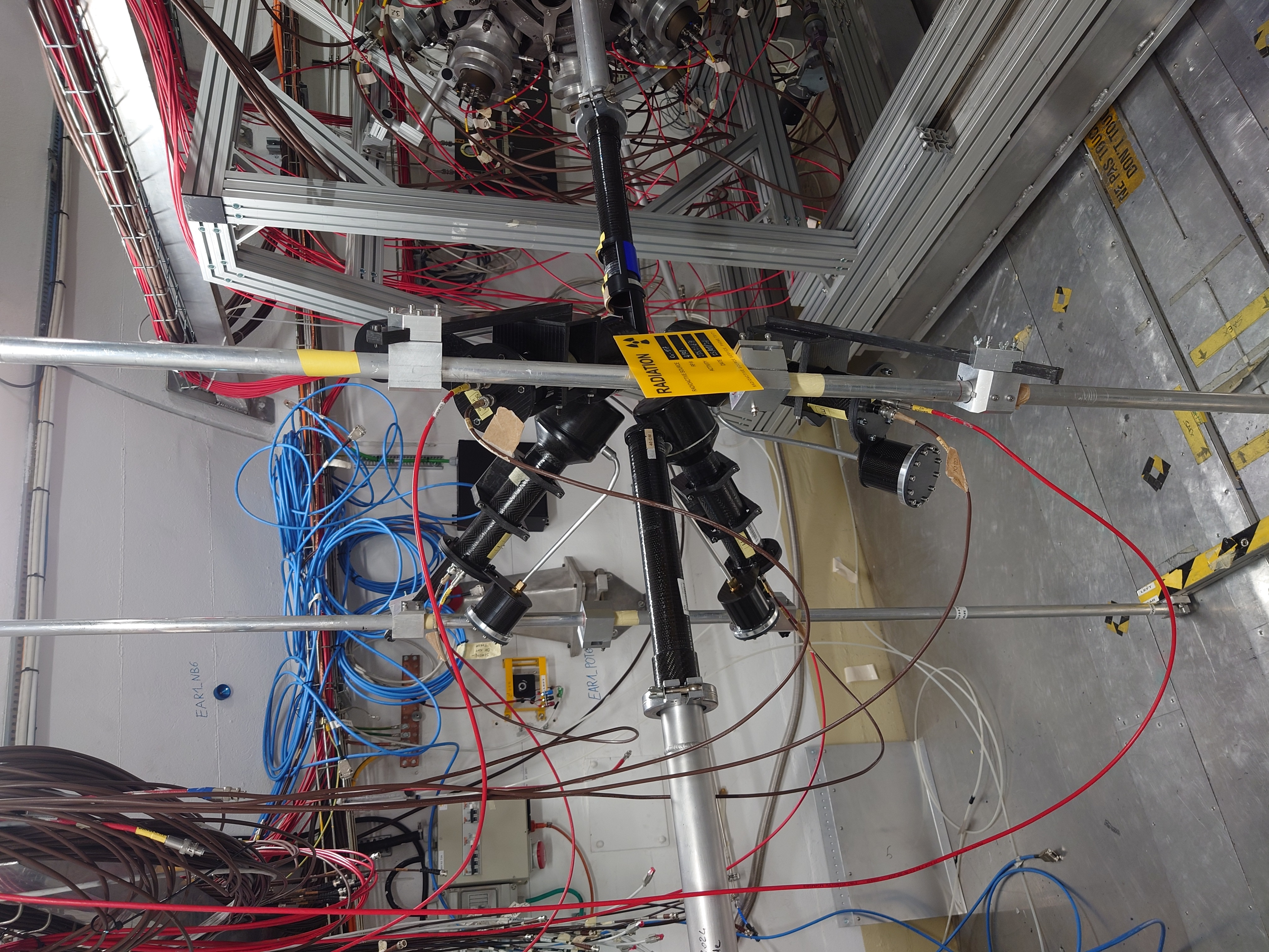
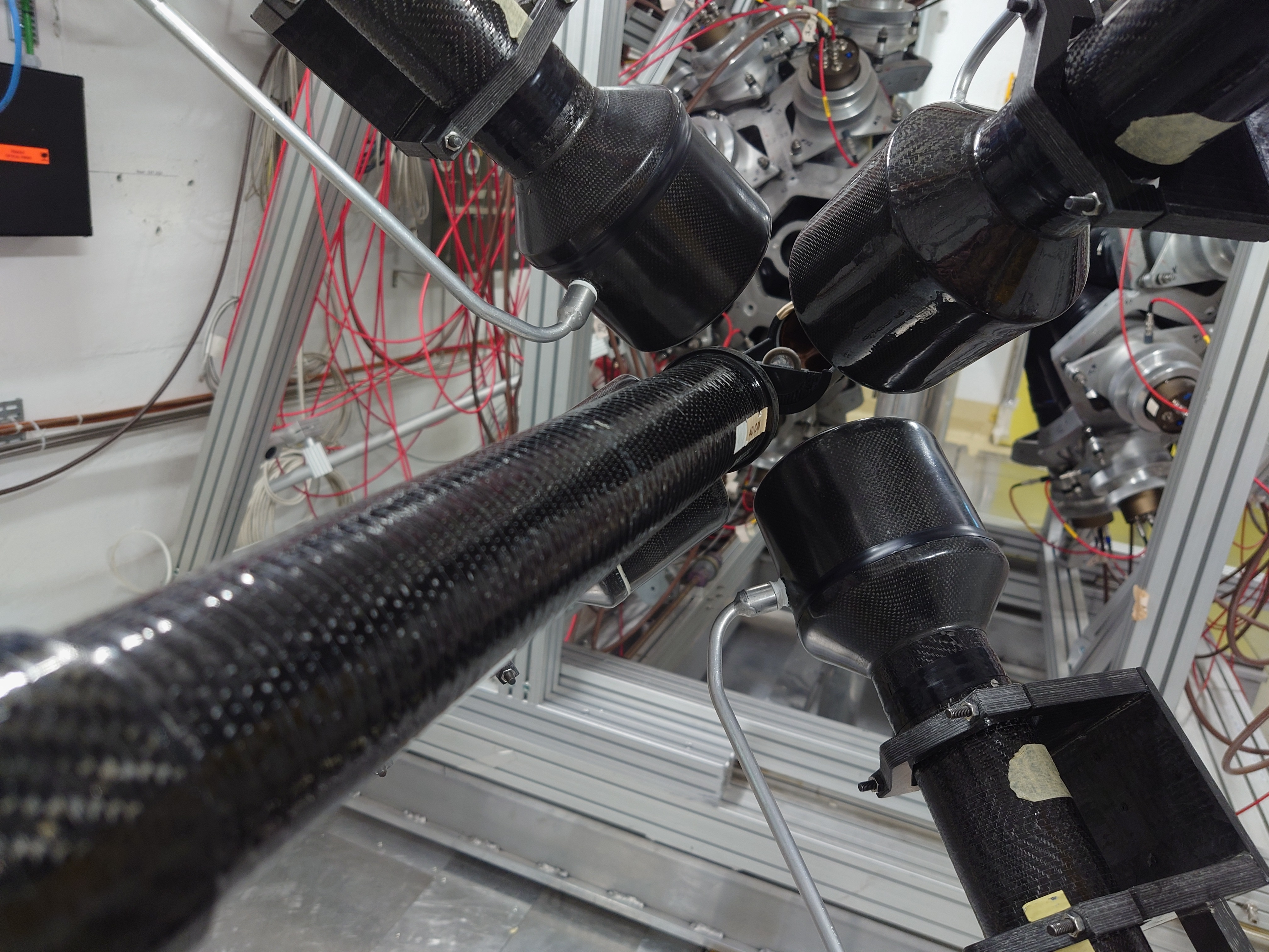
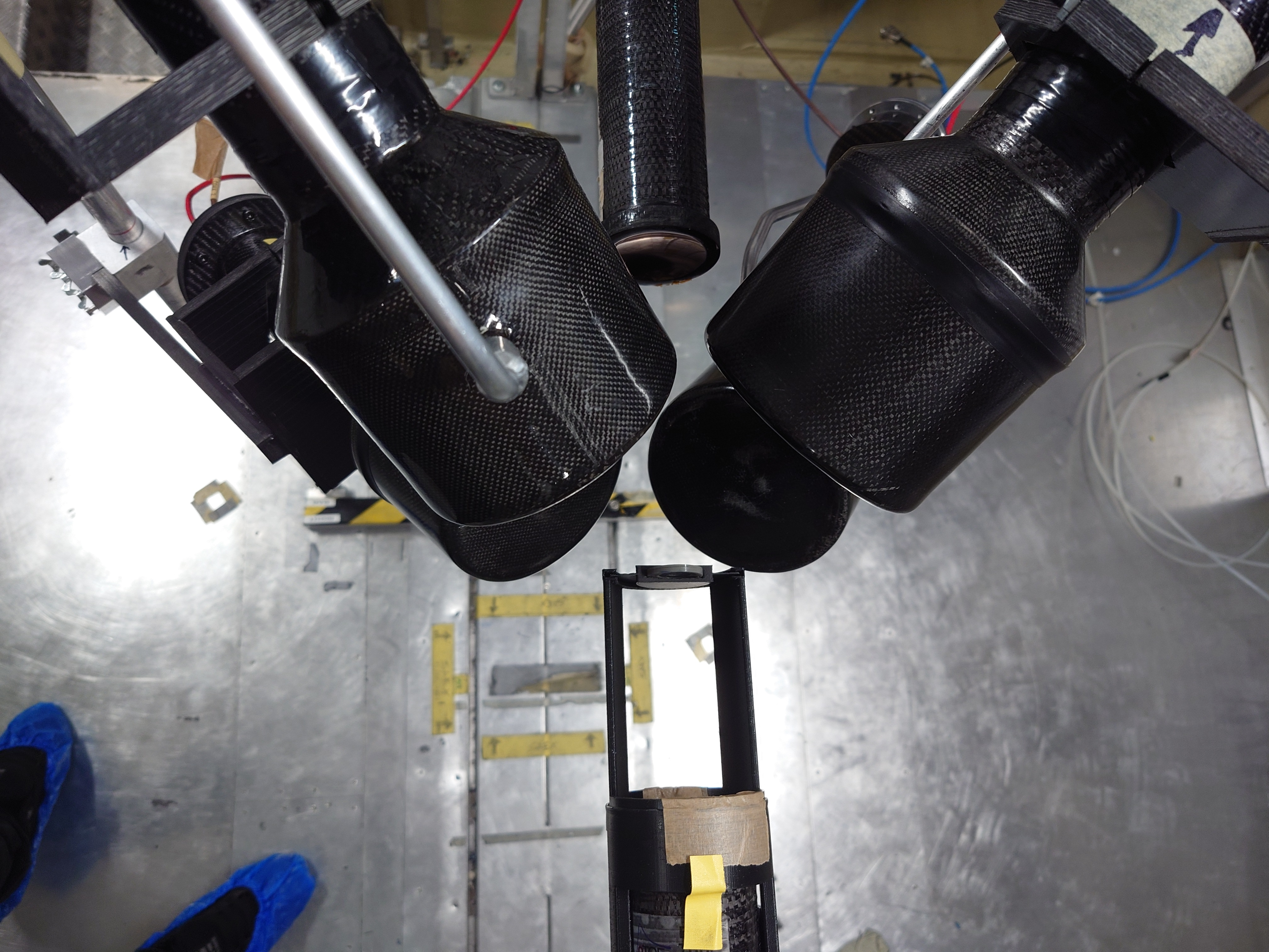
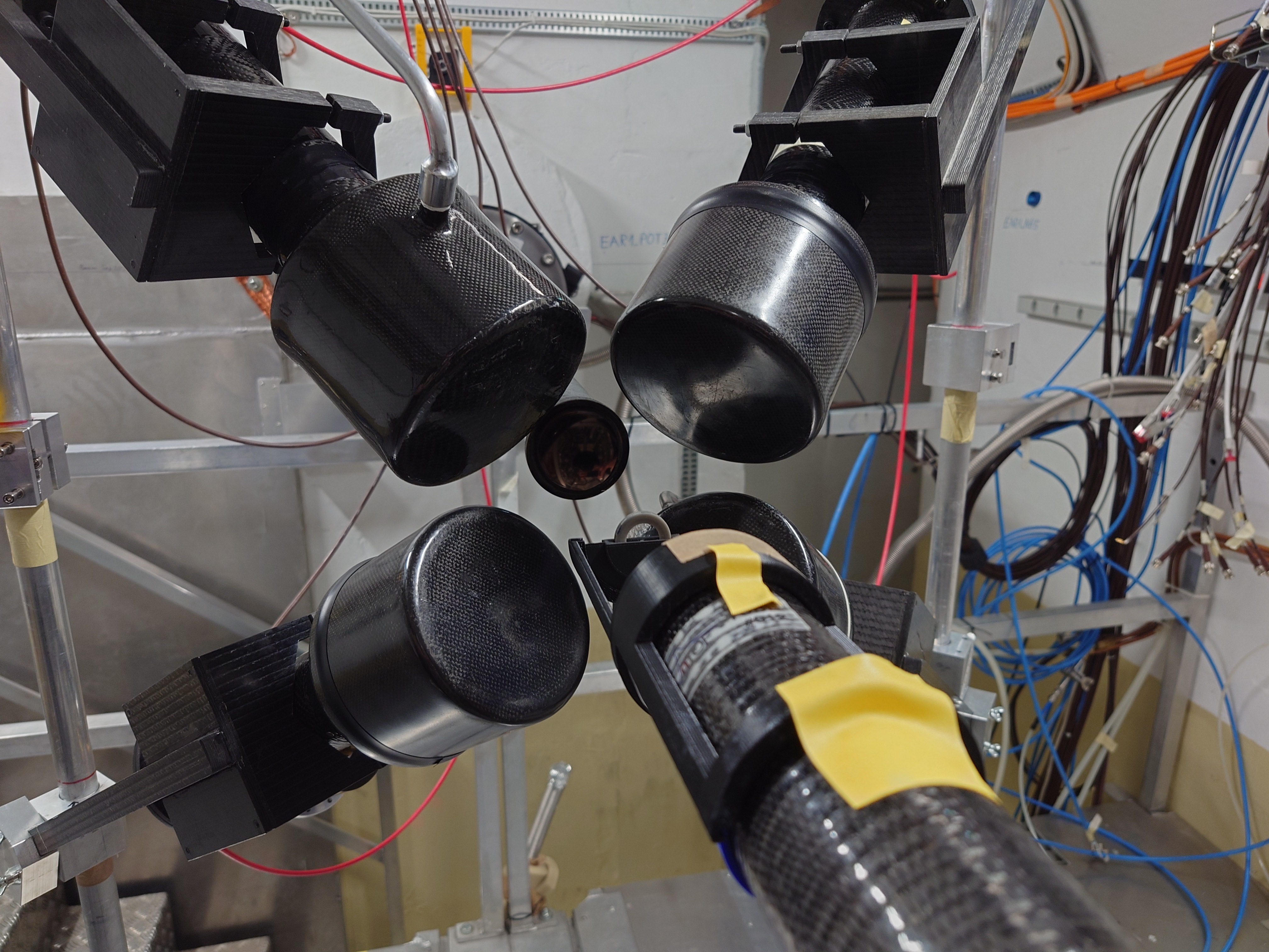
Nick | Detector Setup - 28/29Si Campaign 2024 |
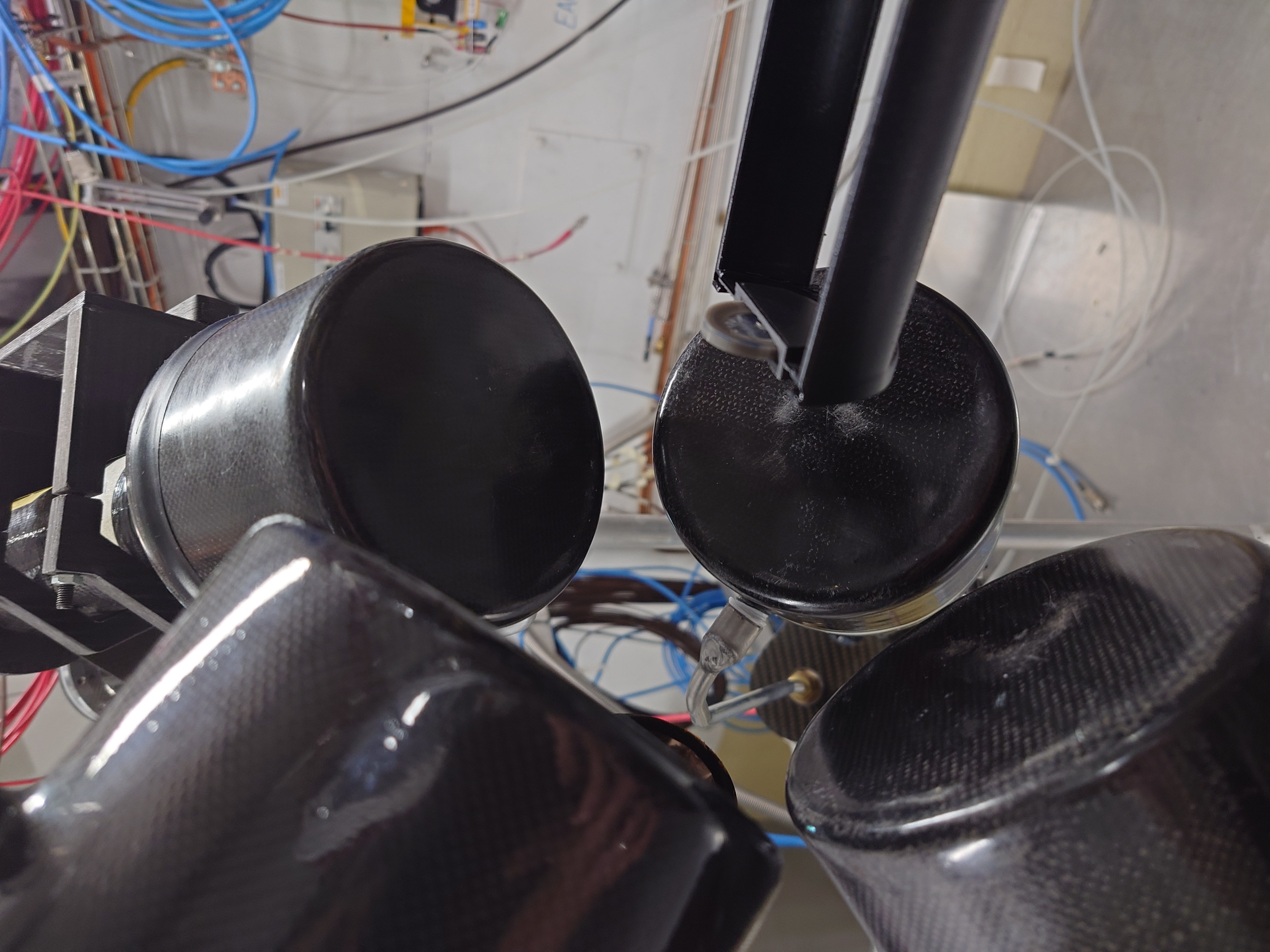
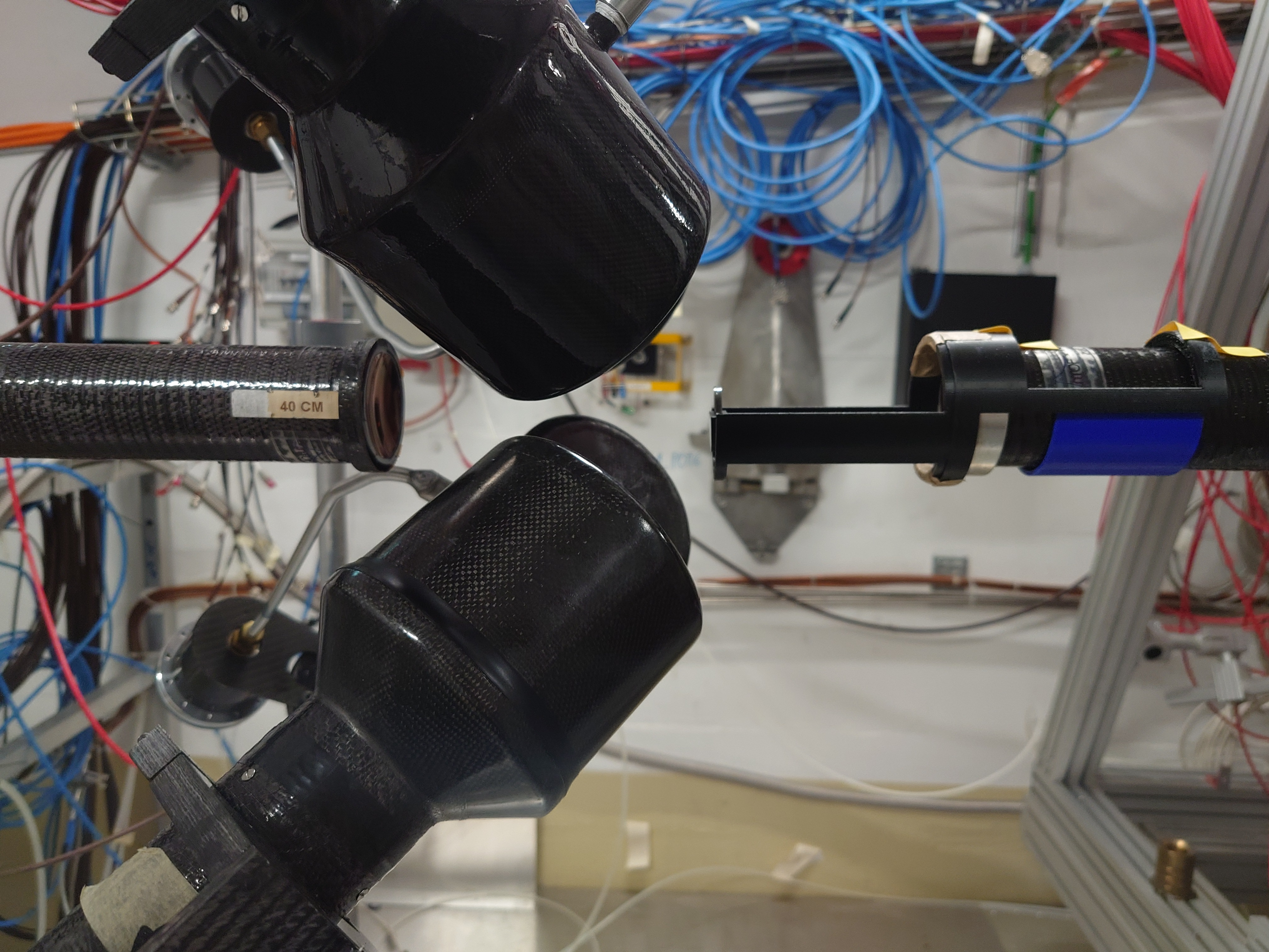
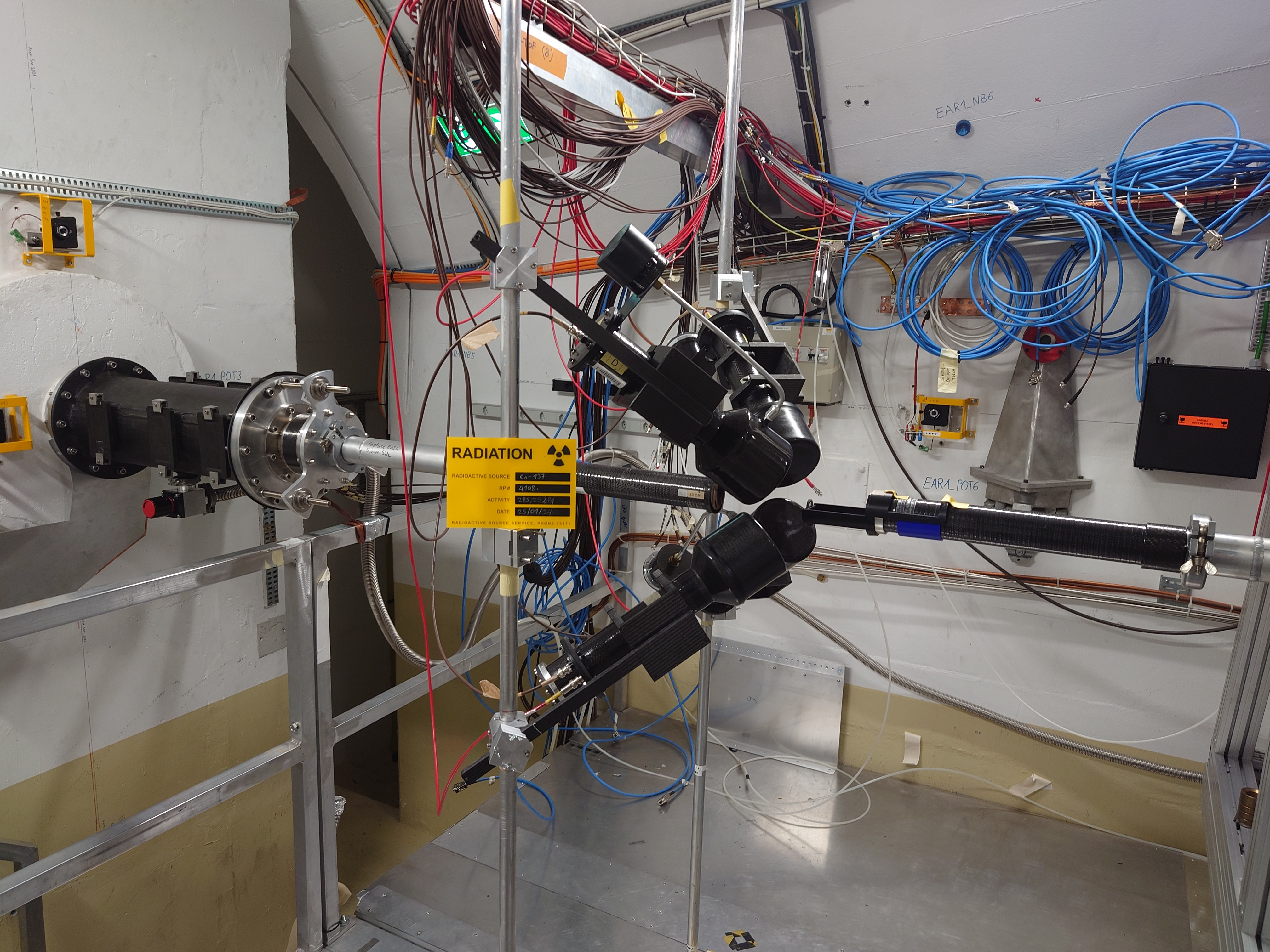
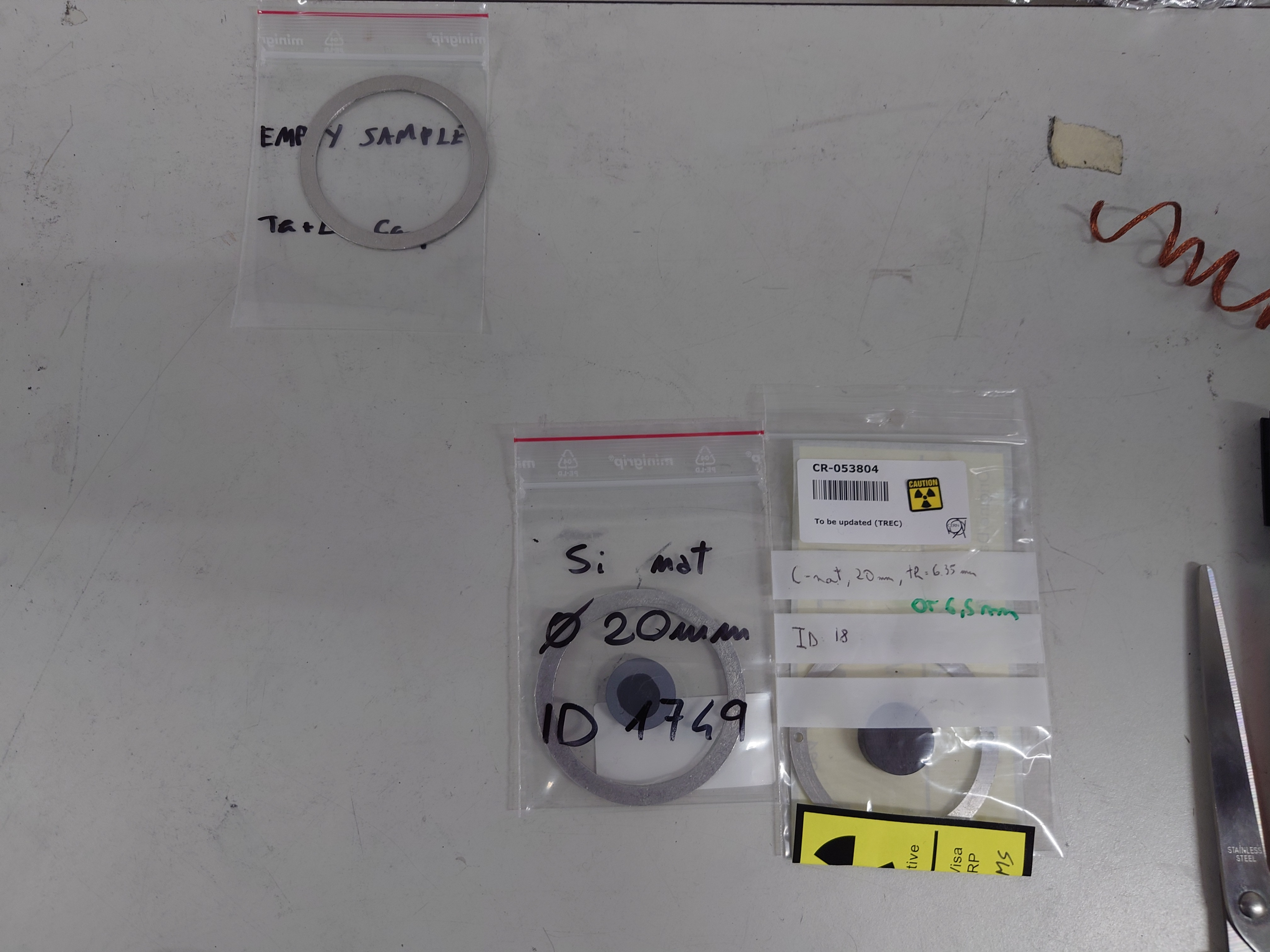
Campaign started yesterday. C6D6s placed at 9 cm distance, angle 125 degrees w.r.t beamline.
Measured calibration sources: Cs137, Y88, AmBe, CmC. Measuring Si-nat over the weekend.
Detector Voltage
| |
|
C6D6_D_1 |
1550 |
|
|
|
|
|
| |
|
C6D6_E_2 |
1590 |
|
|
|
|
|
| |
|
C6D6_H_3 |
1460 |
|
|
|
|
|
| |
|
C6D6_L_4 |
1450 |
|
| Attachment 1: 20240322_145150.JPG
|
|
| Attachment 2: 20240322_144319.JPG
|
|
| Attachment 3: 20240322_144309.JPG
|
|
| Attachment 4: 20240322_144304.JPG
|
|
| Attachment 5: 20240322_144251.JPG
|
|
| Attachment 6: 20240322_144247.JPG
|
|
| Attachment 7: 20240322_144243.JPG
|
|
| Attachment 8: 20240322_144239.JPG
|
|
| Attachment 9: 20240322_144234.JPG
|
|
|
2
|
Fri Nov 3 11:22:43 2017 |
Claudia | Detector Configuration |
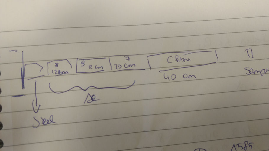
Distance Sample to Detector: Det1: ~10.5 cm, Det2: 11 cm, Det3: 11 cm, Det4: 11 cm
|
| Attachment 1: fig1.jpg
|

|
| Attachment 2: fig2.jpg
|
|
| Attachment 3: fig3.jpg
|

|
|
7
|
Mon Aug 3 14:27:18 2020 |
Nikolay Sosnin | Dead-time and BG Subtraction Meeting Slides |
My TTOFSort macro is located in
/afs/cern.ch/work/n/nsosnin/public/C6D6_Calibration/Calibration_Data/Calibrator.C |
| Attachment 1: Subtracted_Spectra.pptx
|
| Attachment 2: Deadtimes.pptx
|
|
58
|
Fri Dec 1 15:34:01 2023 |
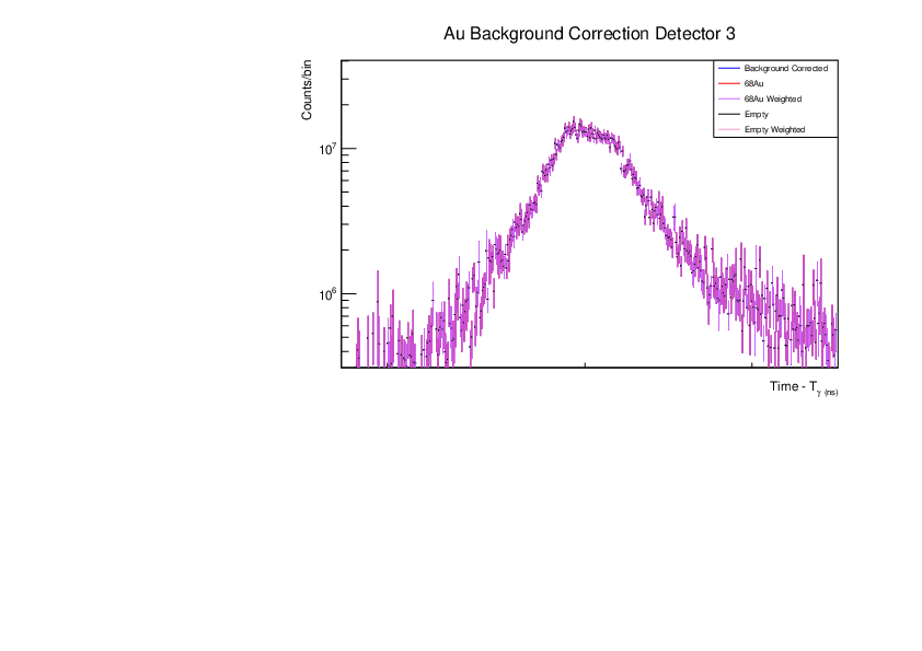
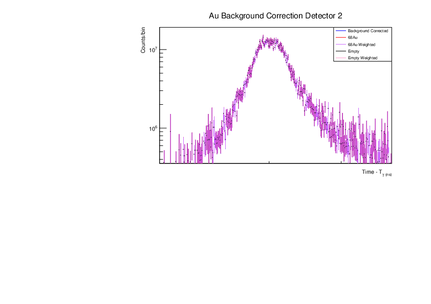
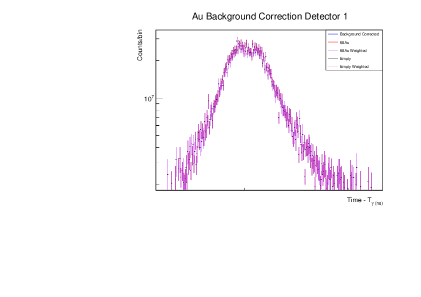
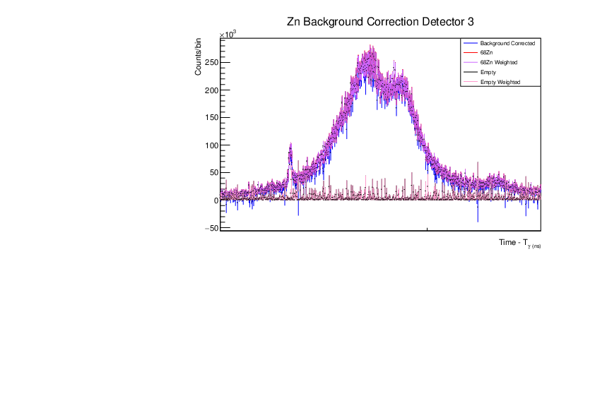
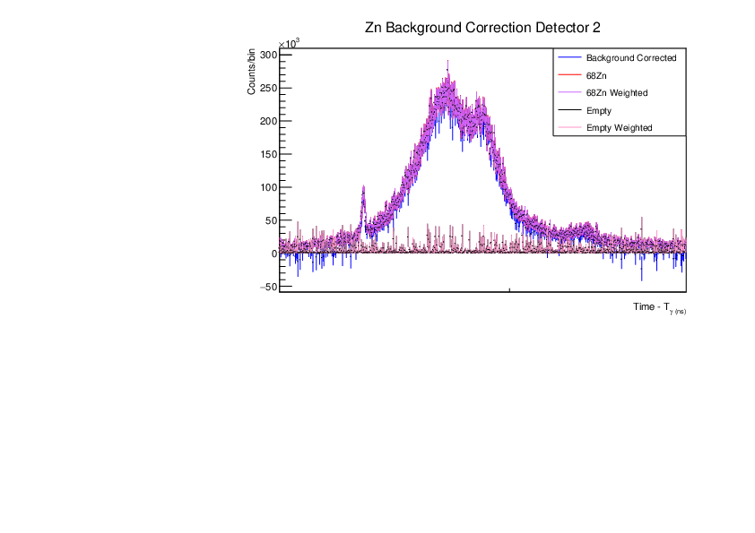
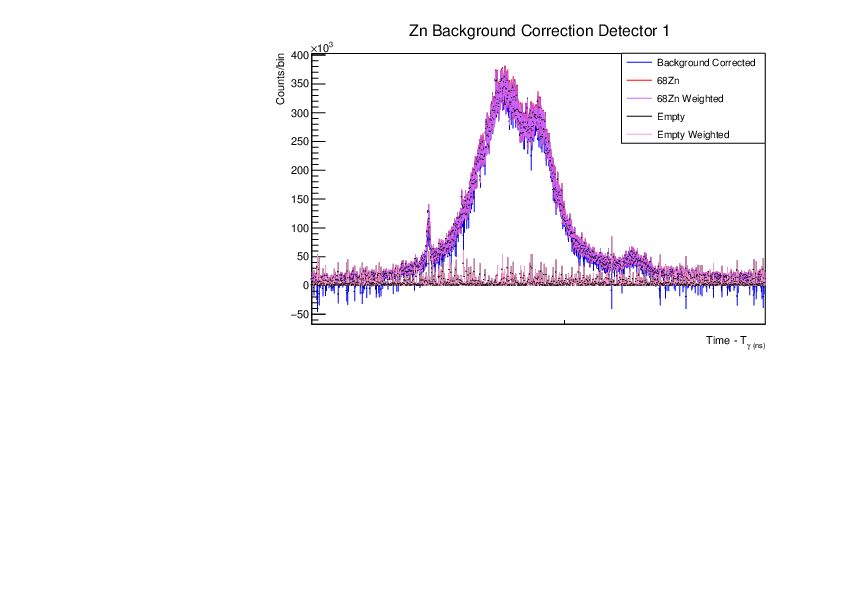
AR | Corrected BG Subtraction plots for Zn and Au |
Updated plots for Zn and Au |
| Attachment 1: Au_BG_correction_comp_weighted_det3_zoomed_rebinned5.pdf
|
|
| Attachment 2: Au_BG_correction_comp_weighted_det2_zoomed_rebinned5.pdf
|
|
| Attachment 3: Au_BG_correction_comp_weighted_det1_zoomed_rebinned5.pdf
|
|
| Attachment 4: Zn_BG_Correction_Comp_Weighted_det3.pdf
|
|
| Attachment 5: Zn_BG_Correction_Comp_weighted_det2.pdf
|
|
| Attachment 6: Zn_BG_Correction_Comp_Weighted_det1.pdf
|
|